
Correlation:
Before entering into Linear Regression let us learn about Correlation. What is correlation? We deal with the problems with the data containing more than one variable. Let us assume that we deal with the data containing the heights of husbands (X) and the heights of wives(Y) at the time of marriage functions. Bi-variate Population is one that is made up of pairs of measurements. It deals with two variables. When we dealing with two sets of data we may raise
the following two questions.
1. Is there any association/relationship with the given two variables. If yes to what extent?
2. Is there any cause and effect relationship between the two variables. That means when one variable increases or decreases does it affect the other variable? If yes to what extent and in what direction
Scatter diagram:
In a bi-variate population you will be having a set of values like (X1 Y1),(X2 Y2), (X3 Y3),(X4 Y4) …(XnYn). You can consider the pairs of numbers as two dimensional co-ordinates and plot the points in X axis and Y axis and get a graph as shown below. This graph is called Scatter Diagram. This scatter diagram reveals two types of information
1. If the variables are related
2. If yes what is the nature of relationship
a)Upward cluster: Increasing trend
When one variable increases, the other variable also increases. Increasing Trend. Positive in the same direction

b) Downward Cluster: Decreasing/Declining
When one variable increases, the other variable decreases. Decreasing Tend. Negative in the opposite direction.Say the price of a car based on the age. As the age of car increase the price of the car will decrease.

c) Curve Linear: Scatter plot show curve linear trend

d) No Relation: Variable Y and Variable X have no relationship with each other. The data points remain in a round shape. Both are unrelated to each other.

CORRELATION ANALYSIS:
It is a statistical technique. Used to describe
- the degree to which the variables are related to each other
- the direction and influence of one on another. The direction could be positive or negative.
- If the increase in one variable is accompanied by the proportionate increase in other then the relationship is called positive correlation.
- If the increase or decrease in one variable is accompanied by the proportionate decreas or increase in other variable then the relationship is called negative correlation


Correlation between two variables: (r)

where:
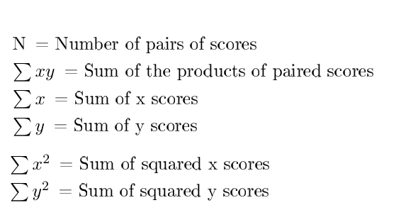
Correlation methods:
- Pearson Correlation
- Spearman Rank Correlation
- Kendall’s Tau Rank Correlation
- Point-Biserial Correlation
- Phi-Coefficient
- Cramér’s V
These methods are used to measure a) the strength and b) the direction of the relationship between variables.
Pearson Correlation:
Description: Measures the linear relationship between two continuous variables.
Usage : can be used only when the variables are continuous in nature and normally distributed.
Range : Correlation r falls in between -1 and +1.
Strength: Simple and most widely used method. Provides linear relationship.
Limitation: This method is sensitive to outliers. Follows linearity
Spearman’s Rank Correlation:
Description: Measures the strength and direction of the association between two ranked variables
Usage: When the variables are ordinal or not normally distributed
Range: r falls in between -1 and +1
Strength: Non-parametric; useful for ordinal data and non-linear relationships
Limitation: Not accurate as Pearson Correlation method
Kendall’s Tau Rank Correlation
Description: Based on ranks, it measures the strength of association between two variables.
Usage: When dealing with small sample sizes or ordinal data
Range: r falls in between -1 and +1
Strength: Most robust with small samples. Accounts for ties in ranks
Limitation: Not powerful for a large datasets
Point-Biserial Correlation:
Description: Measures the relationship between a binary variable and a continuous variable.
Usage: When you have one binary variable and one continuous variable.
Range: r falls in between -1 and +1
Strength: Suitable for finding relationship between one binary variable and one continuous variable
Limitation: Applicable to binary variable
Phi Coefficient:
Description: Measures the association between two binary variables.
Usage: When both variables are binary.
Range: r falls in between -1 and +1
Strength: Useful for binary data; interpretable in terms of contingency tables.
Limitation: Limited to binary data
Cramér’s V Correlation:
Description: Measures association between two nominal variables
Usage: When both variables are categorical (nominal).
Range: r falls in between -1 and +1
Strength: Useful for categorical data; provides a measure of strength of association
Limitation: not suitable for interpretation when you compare this with other methods
Choosing the Right Method
- Continuous Variables: Use Pearson if the data is normally distributed, or
- Spearman/Kendall if the data is not normally distributed or is ordinal.
- Binary Variables: Use Point-Biserial for one continuous and one binary variable,
- Phi for two binary variables.
- Categorical Variables: Use Cramér’s V for two nominal categorical variables.
Choosing the right one depends on the type of data you have on hand
Explanation
- Pearson Correlation: This is the most commonly used method. It calculates how well the relationship between two variables can be described by a straight line. Values range from -1 (perfect negative correlation) to +1 (perfect positive correlation), with 0 indicating no correlation.
- Spearman’s Rank Correlation: Instead of raw data, it uses ranks (e.g., 1st, 2nd, 3rd) to determine how well one variable can predict the other. It’s more flexible than Pearson and works well with non-parametric data (data not normally distributed) and ordinal data.
- Kendall’s Tau: Similar to Spearman’s but calculates correlation based on the idea of concordant and discordant pairs. It’s often used with smaller datasets and can be more robust when there are tied ranks.
- Point-Biserial Correlation: This is used when you have one binary variable (e.g., yes/no) and one continuous variable (e.g., height). It measures how the continuous variable differs across the binary categories.
- Phi Coefficient: This is used when both variables are binary (e.g., presence/absence). It’s useful in contingency tables to measure how strongly the two binary variables are related.
- Cramér’s V: This is an extension of the Phi coefficient for categorical variables with more than two categories. It measures the strength of association between nominal variables.
Pearson Correlation:
Example:
Find out the correlation coefficient (r) for the following data


Second method:


Given two variables x and y are positively correlated.Good relationships exists as r works out to 0.83 closer to positive one. r lies in between -1 and +1.
Using Excel:

Open excel –> Go to Data tab –> Select Data Analysis
Data Analysis popup will appear; Select Correlation option; press OK

Correlation popup appears; in input range box select the range of data. Here A1:B8. It will appear in the box as $A$1:$B$8; Next grouped by select columns option. Tick the labels in the first row. meaning you are instructing the system that first row contains labels only and no numericals. In output options select the output range. could by in the same worksheet or a new worksheet or in the new workbook. Now you press ok

Correlation works out to 0.83355

Covariance(x,y) = 128.15
Descriptive Statistics:

open excel >> Data >> DataAnalysis >> Descriptive Statistics

in popup (Descriptive Statistics) select input range A1:B8 will appear as $A$1:$B$8. Grouped by columns. Tick labels in first row option. Give output range, Tick Summary Statistics, Confidence Level of mean to 95 % kth largest and smallest and press ok


Visualization in Excel


Standard Error:
- Now we can measure the strength of relationship between two variables
- We can estimate the value of one variable when we know the value of other variable
- Our estimation is based on the line of best fit.
- However, some error may come
- Standard Error of Estimate is a measure which points out the error.
- A small Se indicates that our estimate is accurate
- Confidence level 65% when actual value of y falls between ybar-Se and ybar+Se
- Confidence level 95% can be achieved when the value of yfalls between ybar-2Se and ybar+2Se

StandardError:
In the previous example we found out
n=7
Sumofy2=26463
Sumofxy=28469
Sumofy=427
a=4019
b=03222

Result and Conclusion:
- We had estimated the value of y as 62.74 when x=70
- Se works out to 5.08
- The actual value of y may lie between 62.74-5.08=57.66 and 62.74+5.08 = 67.82 when x=70
- A95% level confidence interval would be(57.66,67.82)
Coefficient of Determination: R^2
It is a measure that provides info about the goodness of fit of a model. When we talk about regression, we talk about R^2. It is a statistical measure that discloses how well the regression line approximates the actual data. When
a statistical model is used to predict future outcomes/ in the testing of hypothesis we use this measure R^2, an important measure. We use the following three sum of squares metrics


Coefficient of determination R^2 enables you to determine the goodness of fit. It is measured in percentage. Takes a value from 0 to 1. The chosen model explains 69.48 % of changes of y for every one unit of change in x. Slope (b) reflects the change in y for a unit change in x.
Adjusted R^2:
- R-squared will always increase when a new predictor variable is added to the regression model. This is a drawback
- Adjusted R^2 is a modified version of R^2
- It adjusts the number of predictors in regression model
- Adjusted R^2 is a modified version of R^2
Calculated as under:

Using R:
The same problem:


Result:

Prediction of dependent variable y When x = 70

Summary:

Visualization:
> #Plot the chart
> plot(y,x,col=”blue”,main=”Import & Export Regression”,
+ abline(lm(y~x)),cex = 1.3,pch=16,xlab=”export in crore”,ylab=”Import in crore”
