When we create a machine learning model, we assume that all features (Independent Variables X) contribute equally to the prediction of model (dependent variable y). But in reality, it is not so as we deal with features of different magnitude. Feature scaling is a transformation technique with which we transform all features to a similar range. We use different techniques for transforming all the features.
Why should we to use scaling/normalization technique?
Say distance- based machine learning algorithms like KNN(K-Nearest Neighbor), Hierarchical Clustering rely on magnitude of the features. Features with the higher magnitude(scales) might dominate the rest of the features in the dataset and affect the accurate prediction. The presence of outliers leads to skewed relationship. Normalization/scaling enables you to remove the outliers. This technique improves the interpretability. You can compare any features of the dataset and get the correct insight.
You may be aware that the pre-processing is an important step in machine learning. Before feeding a dataset in data modeling we have to use two common techniques for feature scaling
- Standardization
- Normalization
Normal Distribution
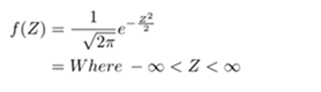
Both of them adjust the feature data into specific range or scale so as to have distinct impacts on model performance. While studying Continuous Probability Distribution we might have come across with normal distribution. A probability distribution which has the following probability density function (pdf) is called normal distribution. It is a bell-shaped curve.
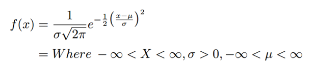
Where
x is continuous. Called Normal Variate. Normal distribution has two parameters µ and sigma. Here π = 3.14 and e= 2.718. mean E(X)= µ, VAR(X) = sigma^2 and SD(X) =sigma
Characteristics of Normal Distribution:
a. Continuous probability Distribution
b. Probability Density Function is given by
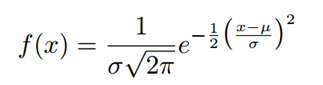
c. Mu and sigma are the parameters
d. It is bell-shaped and symmetric about its mean
e. It is symmetrical on both sides (not skewed)
f. The mean, median and mode are equal
g. Mean divide the curve into two equal parts
h. The quartile deviation QD = 2/3 σ
i. The mean deviation MD = 4/5σ
j. The X-axis is asymptote to the curve
k. Asymptote is a straight line that touches the curve at infinity
l. The mean, median and mode coincide
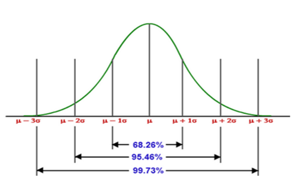
m. Symmetrical bell-shaped curve is divided into two equal parts with mean in the middle with mean plus/minus sigma
Standard Normal Distribution:
Normal variate (X) can be converted to Standard Normal Variate (Z) by substituting mean as zero and sigma as 1 in the original formula
The probability density function of standard normal variate Z is given by
Problem: Data of marks are given below in excel:
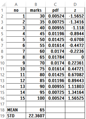
Mean of marks works out to 65
Std of marks works out to 22.3607
pdf of marks is calculated using NORM.DIST(B2,Mean,STD,FALSE). Extend the result to C16
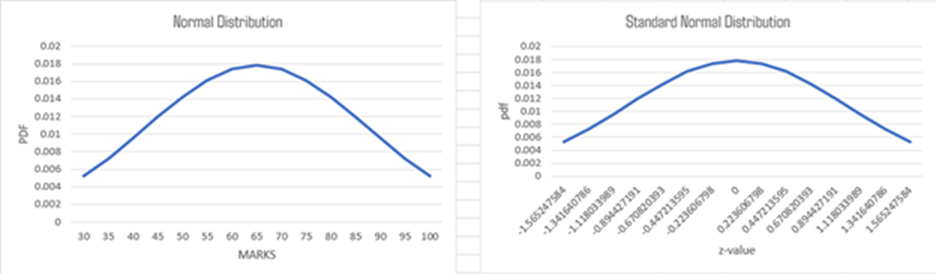
Then you can insert line graph and go to Select Data button and click. you can draw normal distribution curve for original data of marks.
You can also calculate Z values for the original marks and draw standard normal distribution curve
Characteristics of Standard Normal Distribution
- Z is a standard Normal variate. To find any probability of X we can use standard normal variate (Z)
- Any normal distribution can be converted into a standard normal distribution
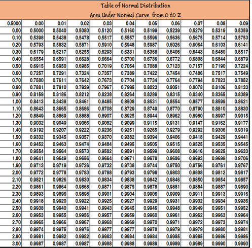
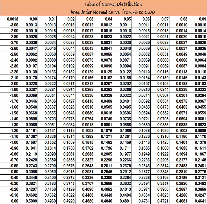
- Area can be read from the table of areas under standard normal curve
- Let X be a normal variate with mean µ and standard deviation σ
- Then Z is a standard normal variate
- Find Z using
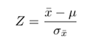
- Standard Normal Variate is denoted by N(0,1)
- Statisticians have developed Standard Normal Table Values
- Z varies from-∞ to +∞
- The mean of standard normal distribution Is 0 and SD is 1
Advantage of Standard Normal Variate(Z):
You can find the Probability of any value of X using Standard Normal variate Z after conversion of X. Let us explain this using one example problem.
Problem:
The weight of Halwa packed by the filling machine follows a normal distribution with mean weight of 500 gm and standard deviation of 10 gm. A pack is selected at random. What is the probability that
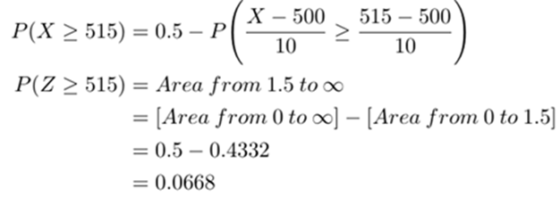
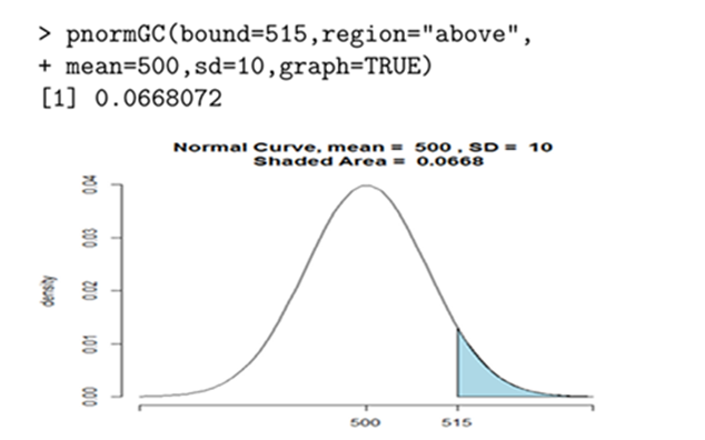
(a) The pack’s weight will exceed 515 gm?
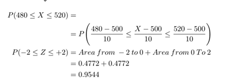
(b) The pack’s weight lies within 480 and 520 gm?
(c) The proportion of packs will have less than 480 and greater than 520 gm
if 10000 packs are supplied how many packs will be rejected given that 480 gm and 520 gm are lower and upper limit for acceptance?
Solution:
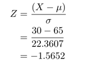
X is normal variate with parameters mean= 500 and standard deviation =10.Therefore Z, the Standard Normal Variate is found out by using
a) Probability that the pack’s weight will exceed 515 gm is given by
Using R based on normal distribution
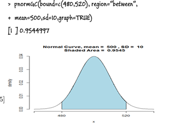
b) What is the probability that the pack’s weight lies within 480 and 529 gm
Using R based on normal distribution
Probability of Rejection:
If the weight lies outside these values, then it will be rejected. The probability of rejection = 1- 0.9544=0.0456 The number of packets that will be rejected is given by
N ∗P =10000∗0.0456 = 456
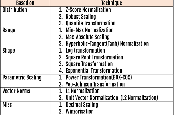
Normalization Techniques: