
Exploratory Data Analysis:
It is the process of analyzing the collected or given data. Before we undertake any predictive and prescriptive analyses, we are supposed to summarize the data and must learn the characteristics of the features, anomalies, hidden patterns, and relationships between the variables/features we handle. We can also identify the patterns using Data Visualization. This is the first step in a Data Science project
For effective model building and further analysis, we have to pre-process the given data. The important tasks we undertake in EDA are
- Finding out the features present in the data
- Finding out the size and shape of the features (df.shape)
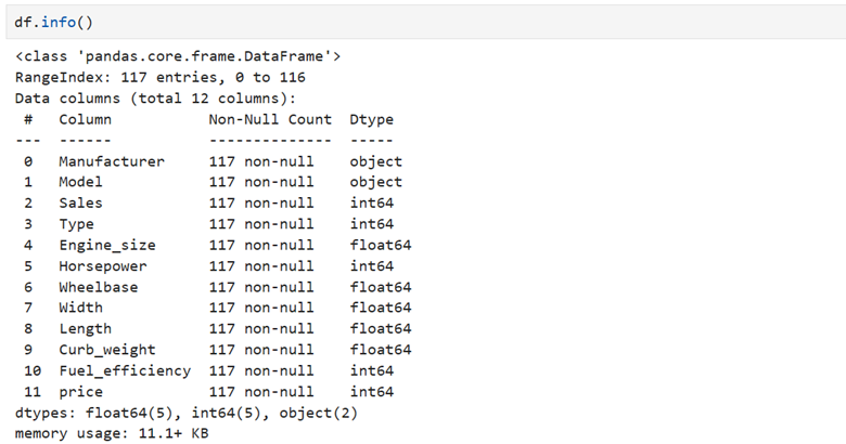
- Finding out the data types of each column(df.info())
- Finding out the descriptive summary of the dataset (df.descriptive ())
- Finding out the missing values (df.isnull().sum())
- Encoding the labels using LabelEncoder()
- Finding out the distribution of the dependent/response/target variable
- Grouping the data based on the target variable
- Data Visualization
- Drawing Distribution Plot for all columns
- Drawing Count plot for categorical columns
- Draw pair plot
- Finding out Outliers (data points below and above 25% quartiles and 75% quartiles)
- Outliers are dangerous which may mislead our output and our model credibility.
- Draw correlation matrix
- Draw meaningful inferences from EDA
Key components of eda
- Descriptive Statistics: We summarize and describe the main features of the dataset.
- Data Visualization: We use various plots like histograms, scatter plots, box plots to see the distribution and relationship between variables.
- Correlation Analysis: In order to determine how variables are related to each other we use this.
- Outlier Detection: This is important. We have to identify unusual observations in the dataset.

1. LOAD LIBRARIES:
This is the first step. Import the necessary python libraries
Pandas library enables you to create dataframes by reading data files with extension csv, xls, xlsx,sql etc. You can also write the dataframe into csv,xls,xlsx or to databases like postgresql, mysql, oracle etc
2.Read Data
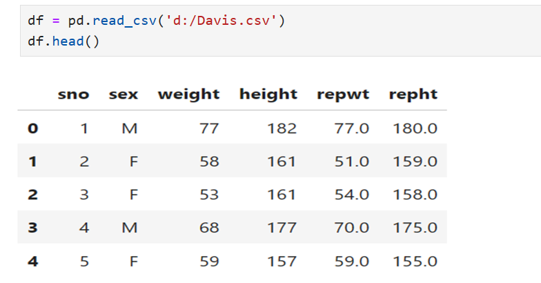
pd.read_csv() is used to read a csv file (comma separated values) in pandas. This converts the file into a Pandas data frame. The function reads data from ‘Davis.csv’ and assign the values to a variable df. Either the value of df can be printed using print(df) or you can view the first 5 rows of the data using df.head()
pd.read_csv() has arguments like sep, header=0, index_col=0
df1 = pd.read_csv(‘d:/Davis.csv’, sep=’,’ , header=0, index_col=0,skiprows=5,na_values=’NAN’)
In the above said case separator is “,” , the first row is the header, the first column is an index,the first 5 rows are skipped and na values are replaced by ‘NAN’.
df.tail(): displays the last 5 rows of the data

3. View the Datatype of each feature
df.info() is the method used to get the summary of the data frame. Displays number of non null values of each column, data types of each column

4. Data characteristics & summary: Here you know the count, mean, standard deviation, minimum, maximum, First Quartile, Second Quartile (median), Third Quartile of each column
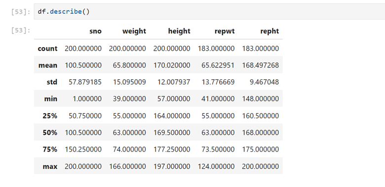 4 a) df.descrbe(include = ‘all’). This includes all columns(even categorical columns besides numerical columns)
5. Shape of the data: Number of rows and columns of the data frame
This table contains 200 rows and 6 columns

6. Find duplicate values if any

# Removing duplicates
df = df.drop_duplicates()
7. How to deal with the missing values?
- Identify the missing data
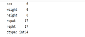
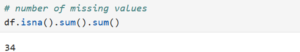
- Find missing values

17 values are missing in the column reported weight and 17 values are missing in the column reported height
![]()
Find values not available (na) in data frame
Find the total number of missing values in the data frame
B) Deal with the missing data
Two options are available to maintain the credibility of the data collected. Drop and Replace
- Drop the data
- a)Drop the entire row if any value is missing in the Target/dependent column. The reason is that our prediction may go wrong if any value is missing in target column b) Drop the entire column if independent variable cells are missing
- Replace the data
- a)Replace the missing value by mean/median/mode
- b)Replace the missing value by frequency
- c) Replace the missing value based on other functions
Dropping entire row if any value is missing in the Target variable column:
# Our prediction may go wrong if we do not drop all rows of dependent variables. Let us assume in data ‘Price’ is the dependent variable and some rows are missing. If we try to predict the regression line with the missing rows it may lead to the wrong equation. What we have to do is
- First drop the rows of the Price column using ‘dropna()’. Use subset
df.dropna(subset=[“Price”],axis=0,inplace=True)
2. Reset index because of the dropped rows
df.reset_index(drop = True, inplace=True)
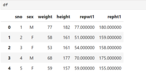
Here in repwt and repht we have 17 missing values.
Let us replace the missing value by the mean
- Calculate the mean of repwt and repht first

![]()

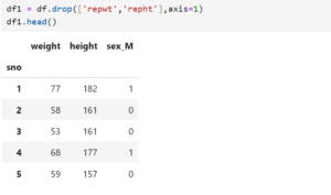
2. Remove the original columns repwt and repht (which contains missing values)
![]()
# replace NAN with mean value in a particular column
df[‘column name’].replace(nan,df[‘column name’].mean(),inplace=True)
df[‘column name’].isnull().sum()
OUTPUT: 0
8. Replace by frequency
Let us assume that we use car.csv file where the ‘number_of_doors’ column contains ‘four’ and ‘two’. Let us assume that under the number_of_doors column, a lot of missing values are found. Normally Car will have four doors. So let us replace the missing value with ‘four’
- First using value_counts() find the numbers
df[‘number_of_doors’].value_counts()
output: four 200
two 163
Name: numberofdoors,dtype: int64
2. Second using idxmax() find out the idxmax
df[‘ number_of_doors’].value_counts().idxmax()
output: ‘four’
3. Now replace by frequency four
# replace by frequency four
df[‘ number_of_doors ‘].replace(np.nan,”four”,inplace=True)
- Additional tips for missing values
# if your data contains’?’ mark in some cells you can replace them using NAN
df1= df.replace(‘?’,NAN)
## Handling missing values
df = df.dropna() # Or df.fillna(value)
#Fill NaN values of ‘Age’ column as mean value.
df[“Age”].fillna(df[“Age”].mean())
#Fill NaN values of ‘Age’ column as median value.
df[“Age”].fillna(df[“Age”].median())
#Fill NaN values of ‘Age’ column as 0.
df[“Age”].fillna(0)
#We can do filling NaN values for each column by using apply and lambda
#If columns is numeric, then fill NaN values as mean value.
dff = df.apply(lambda x: x.fillna(x.mean()) if x.dtype != “O” else x,axis=0)
Data Reduction
Dropping Irrelevant Columns: Identify and remove columns that don’t contribute to the analysis or predictive modeling.
Handling Constant Columns: Remove columns with constant values as they don’t add any value.
df = df.drop([‘irrelevant_column1’, ‘irrelevant_column2’], axis=1)
df= df.loc[:, df.apply(pd.Series.nunique) != 1]
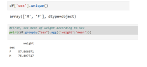
10. Find Categorical Variables Option
The column ‘sex’ contains two options 1) ‘M’ and 2)’F’

Example 2:


11. Categorical Variables & Groupby function


#catagorical variables
catcols = [‘column name’,’column name’,’column name’,’column name’,’column name’]
for col in catcols:
categories = df.groupby(col).size()
print(categories)
12. If your data do not have column headers you create column headers
col_names = [‘column name’,’column name’,’column name’,’column name’,’column name’]
df.columns = col_names
df.head(0)
13. Creating new columns using existing columns in a data frame
# Creating a new column based on existing data
df[‘new_col’] = df[‘existing_col_1’] / df[‘existing_col_2’]
14.How to r emove non-numeric characters like $ , etc found in your data?
# removing non numeric characters like $, comma from the data frame
df[‘column name’] = df[‘column name’].astype(str).str.replace(r'[$, ],”,regex=True).astype(float)
df[‘column name’] = df[‘column name’].astype(str).str.replace(r'[%, ],”,regex=True).astype(float)
15. Convert text to lowercase
df[‘Text_Column’] = df[‘Text_Column’].str.lower()
16. Extract information using regular expressions
df[‘Extracted_Info’] = df[‘Text_Column’].str.extract(r'(\d+)’)
17. Convert date to datetime object
#convert date to datetime object
df[‘date’] = pd.to_datetime(df[‘date’])
18. Extract month and year from a datetime column
df[‘Month’] = df[‘Date’].dt.month
df[‘Year’] = df[‘Date’].dt.year
19. Sum of a column
#find total income
totalincome = df[‘Total income’].sum()
totalincome
20 Statistical measures
meanval = df[‘column name’].mean()
medianval = df[‘column name’].median()
modeval = df[‘column name’].mode()
varval = df[‘column name’].var()
stdval = df[‘column name’].std()
rangeval = df[‘column name’].max()-df[‘column name’].min()
iqr = df[‘column name’].quantile(0.75) – df[‘column name’].quantile(0.25)
skewness = df[‘column name’].skew()
kurtosis = df[‘column name’].kurt()
21. Merge data frames
# Load another dataset
df_additional = pd.read_csv(‘additional_data.csv’)
# Merging datasets
df = pd.merge(df, df_additional, on=’common_column’)
syntax:
df.merge(right, how=’inner’, on=None, left_on=None, right_on=None, left_index=False, right_index=False, sort=False, suffixes=(‘_x’, ‘_y’), copy=None, indicator=False, validate=None)[source]#
Data Frames using series:
Series 1


Series 2

Series 3:

Create Dataframe using the above mentioned three series

DataFrame created using Dictionary


22. Data Formatting
We use
.dtype() to check the data type
.astype() to change the data type
X = X.astype(np.float64)
Y = y.astype(np.float64)
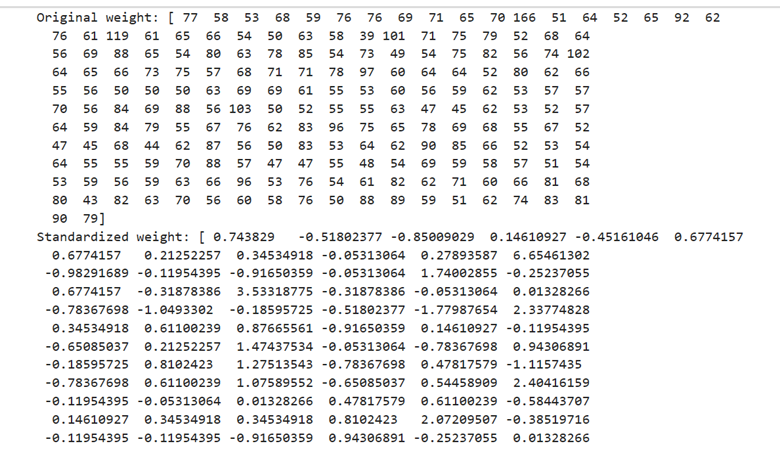
23. Standardization
- dIt is a process of transforming the original data in such a way that the mean of data becomes 0 and the standard deviation of the data becomes 1 just like Standard Normal Distribution where the mean is 0 and the standard deviation is 1
- It enables you to bring different features into a similar scale to make comparison easy.
- It prevents certain features from dominating other features due to their large magnitude

Here height and weight are in different measures. One in centimeters and the other in kg. To make them on a similar scale we use standard scaler(). Under the standardization process the standardized height and the standardized weight will have a mean 0 and a standard deviation 1
Since both standardized height and weight are in the same scale it prevents the domination of one over other


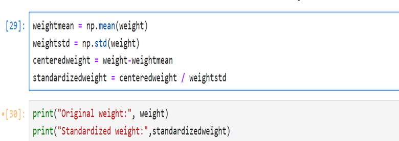
When you want to standardize the fields/features you have to do the following:
- Calculate the mean of the feature
- Calculate the standard deviation of the feature
- Calculate the difference between the mean and individual height or weight
- The above-mentioned step centers the data around 0
- Now divide the centered height by the standard deviation of height
- Now divide the centered weight by the standard deviation of the weight
Example 2


Standardization may look absurd. But it provides many advantages in data analysis and machine learning
- Comparability: the height and weight are measured in different units. When you try to analyze the variability in height and weight it is better to standardize the height and weight for comparability purposes. It ensures the true picture as they have been standardized
- Normalization: Standardization helps to normalize the distribution of the data. When you use Gaussian Distribution, techniques of clustering, principal component analysis normalization improves the data characteristics for further analysis.
- Interpretability: If a coefficient of the linear regression model is larger for a standardized feature it indicates that a one-standard-deviation change in that feature will have a larger effect on the outcome variable compared to other features
- Outlier Detection: Standardization can make outlier detection apparent and easier.
- Standardization is used as a pre-processing step to the quality and performance the mode
24. Normalisation
- It is a process of scaling numerical data into a common range
- Common range normally falls between 0 and 1
- This transformation is useful for the following reasons
- For maintaining proportions: Normalization preserves the proportional relationship within the data when we deal with features having different measures. Under this, no single feature can dominate over others
- Interpretability: Normalized data are more interpretable. You can understand the relative importance of each feature in a dataset
- Focusing on convergence: Normalization of input features may improve the convergences in algorithms like Gradient Boosting Regression, Logistic regression, and neural networks.
- Better Performance: It leads to better performance. For better performance, we use algorithms like k-nearest neighbors and support vector machines where we deal with sensitive features we are supposed to use normalization.


In this example, the MinMaxScaler scales each feature to a given range (by default, between 0 and 1) by subtracting the minimum value and then dividing by the difference between the maximum and minimum values for each feature.
Normalized data can be converted to the original data as follows:

We can normalize the given data falling in the range between 0 and 1. After finishing our analysis we can inverse the scale and get back the original data.
25. Binning
It is the process where we transform the continuous variables into discrete categorical bins for grouped analysis.


Using Univariate analysis you have can get some insights about the range, central tendency disbursion and shape of each variable of the given data
29. Bivariate analysis
Using this you can explore the relationship between two different variables. How they are correlated with each other and the pattern(positive or negative or neutral)


30. Multivariate analysis
Here we examine the relationship among multiple variables simultaneously. We can understand the complex interactions and patterns prevail in the given dataset.


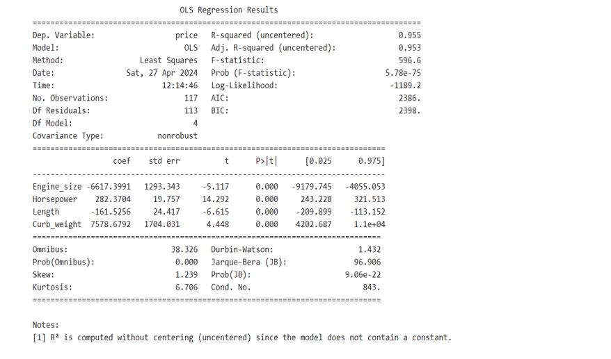
31.Ordinary Least Square using statsmodels.api
Identify dependent variable y and Independent variables X
In this example let out dependent variable y be height
And X be weight, sex.
First drop dependent variable height from X
Then assign datafame[‘height’] to y
Convert dataframe df1 to numpy array
Now pip install statsmodels
Let us import statsmodels.api as some variable (here sm)
lm is linear model.
Now you fit the linear model using sm.OLS(y,X).fit()
Then print lm.summary()


Under the first iteration of Ordinary Linear Squares
Height = 2.6100*weight – 20.0835*sex_M
For Male Height = 2.6100*weight – 20.0835*1= 2.6100*weight – 20.0835
For female height = 2.6100*weight – 20.0835*0 = 2.6100*weight
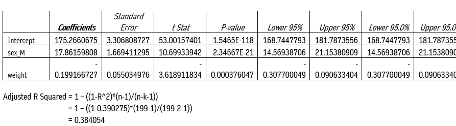
Under IInd iteration: we add constant and find another lm1. Summary


II nd iteration: Equation
Height = constant + b_0*weight+b_1*sex_M
Height = 175.2661 – 0.1992*weight+17.8616*sex_M
For M height = 175.2661 – 0.1992*weight+17.8616*1
For F height = 175.2661 – 0.1992*weight+17.8616*0
= 175.2661 – 0.1992*weight
Conduct IIIrd iteration and examine if any variance occur.


32. Find features patterns using Visualization Technique
After doing the following
- Cleaning
- Finding out the missing values
- Replacing the missing values
You are supposed to find out the patterns of each feature of the data
using Visualization technique
Your individual features could be of type
- Continuous Numerical Variables
- Categorical Variables
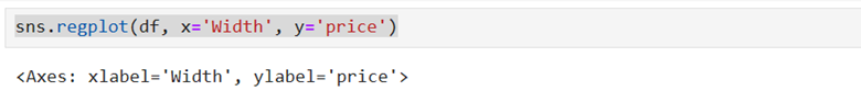
- Continuous Numerical variables: The data points could fall between any two given values or a range. Say Height 150 to 190 cms. Individual data points could assume any value say 150.3, 163.58… Height is not a discrete variable. It can be of type int64 or float64. We can visualize continuous variables using SCATER PLOTS with fitted lines.
Our aim is to understand the relationship(linear) between dependent and independent variables we use regplot of seaborn. It plots the scatter plots along with the filtered regression line for the data.
We come across different linear relationships
- Positive Linear Relationship
- Negative Linear Relationship
- Neutral/no Linear Relationship


a.Positive Relationship


b.Negative relationship


box plot


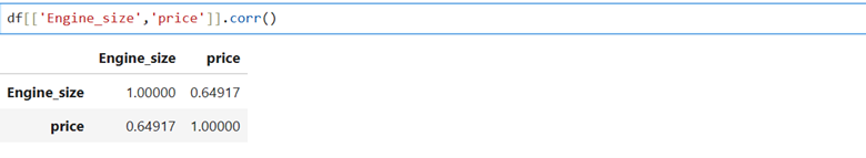
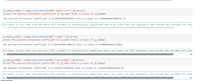
Correlation

Heatmap


Grouping:
0 car 1 Passenger