
Problem 1:
Let us discuss about the problem on hand. We have 50 records of customers containing Purchased as dependent variable y and Gender(Male=1,Female=0),Age, Annual salary as independent/explanatory variables as X1,X2,and X3. Our aim is to predict the probability of a customer who will buy our car using Logistic Regression Model.

purchased is dependent variables. our Logistic Regression assumes
Yi = 0 denotes the customer has not purchased any car from us
Yi = 1 denotes the customer has purchased a car from us.
We are concerned with the probability of the customer who is going to buy based on the info, gender, age and annual salary ( independent variables)

In binary logistic regression the dependent variable (purchased status) can take only two values either 0 or 1
In multinomial logistic regression the dependent variable can take two or more values(but not continuous)
Covariates: All independent (explanatory) variables are entered as covariates in SPSS. Method followed Forward Step-wise Likelihood Ratio (LR forward). While moving forward the system takes age and constant only in the step1 and in the second step it concludes with the parameters found for independent variables like age, annual salary besides the constant (intercept)


The probability of a customer who may purchase a car with us is found using the above-said formula
Using Python:
We use statsmodels.api library. we use sm.logit function and get the following summary

Classification Table using SPSS

Here the cut off value is 0.500
In the first step the overall percentage of correctness works out to 72%. During the second step we get 80% as overall percentage. We have to accept this classification table and to calculate Accuracy, Sensitivity and Specificity and Recall. This also comes under method Forward step-wise LR method. This is also called confusion matrix
Confusion Matrix using Python
Code
In python we use sklearn
#using sklearn
#use sklearn.linear_modelf
from sklearn.linear_model import LogisticRegression
from sklearn import metrics
#instantiate the model
log_regression = LogisticRegression()
#fit the model using the training data
log_regression.fit(X,y)

#use model to make predictions on test data
y_pred = log_regression.predict(X)
#Using confusion matrics we get the following
cnf_matrix = metrics.confusion_matrix(y, y_pred)
cnf_matrix
Output:

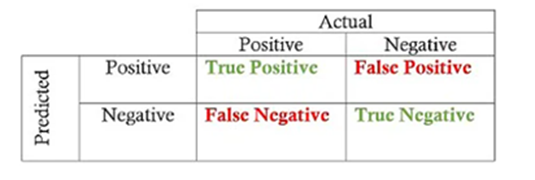
Actuals are shown as rows and predicted are shown as columns:[0 :1,0:1]


When predicted are shown as rows and Actuals are shown as columns : [1:0,1:0]
Formulae:
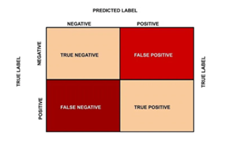
- Accuracy: (TP + TN) / (TP + FP + FN + TN)
- Recall: TP / (TP + FN)
- Precision: TP / (TP + FP)
- F1 Score: (2 * Precision * Recall) / (Precision + Recall)
Accuracy = TP+TN/(TP+FP+FN+TN)
=17+23/(17+5+5+23)
=40/50
= 0.8
Precision = TP/TP+FP
= 17/(17+5)
= 17/22
= 0.77
Recall = TP/TP+FN
= 17/17+5
=0.77
F1_score =2 * (precision*Recall)/(precision+recall)
= 2*(.77*0.77)/0.77+0.77
=.77
Classification Table when cut-off point is set to 0.300

The effect of changing cut-off point
Cut off value is 0.300. When cut off point is reduced to 0.300 from 0.5 Percentage correctness for Purchased changes to 90.9%. A change from 77.3%. Out of 22 customers 20 customers have been correctly classified as TP. The remaining 2 customers have been classified as FN. The overall percentage has changed to 82% from the previous level of 80%. Cut of value can be increased or decreased. When we fixed the cut off value as 0.500 accuracy for the customers worked out to 77.3% and the overall accuracy worked out to 80%. It is better to have the cut off value as 0.3 as the overall accuracy of the model improved to 82%
LN.PARAMETERS
Whether it be Linear Regression model or Logistic Regression mode we have to find the parameters Beta 0, Beta1, Beta2… Beta n. But in Logitic regression,we use different method to find out the same Before that we must know Odds and Odds Ratio. For Logistic Regression model we use Logit function

ODDS
Odds is nothing but a ratio of two probability values

ODDS RATIO
Odds Ratio is nothing but a ratio of two odds. Beta coefficients: Beta not and Beta one
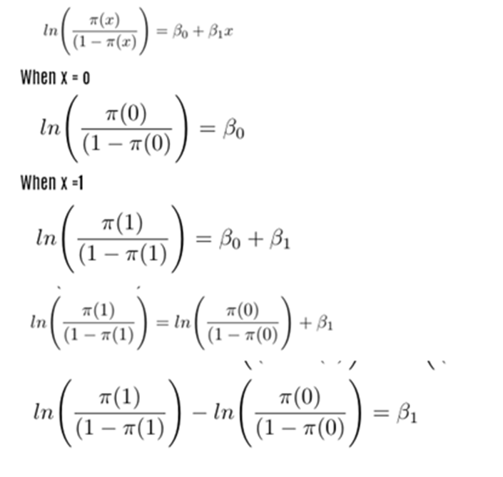
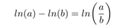
ODDS RATIO
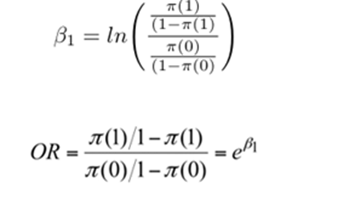
If OR(Odds Ratio) = 2 the event is likely to happen twice when x =1. OR approximates the relative risk. The relative risk either increases or decrease as the value of x increases or decreases. Beta 1 is the change in log odd ratio for a unit change in the explanatory variable. Beta 1 is the change in odd ratio by the factor exp(B1)
Calculation of Odds ratio, Lower Confidential Boundary and Upper Confidential Boundary based on confusion matrix


odds (not purchased) = a/c = 23/5 = 4.6
odds (purchased) = b/d = 5/17 = 0.294118
odds ratio = 4.6/0.294118 = 15.64
ln(OR) = LN(15.64) = 2.749831735
Upper CI =4.138947482
lower CI =1.360715988
LCB = e^(1.361) =2.71828^(1.361) =3.898980
UCB = e^(4.139) = 2.71828^(4.139) = 62.73658044
Log Odds Ratio

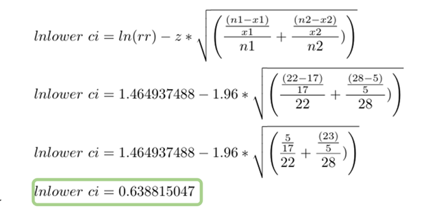
Odds = a/c = 23/5 = 4.6 = TN/FN
Odds = b/d = 5/17 = 0.294118 =FP/TP
Odds ratio = (a/c)/(b/d) = 4.6/0.294118 = 15.64
Ln(OR) = ln(15.64) = 2.749831735
Upper CI = ln(OR) + 1.96 * Sqrt(1/a+1/b+1/c+1/d)
= 2.749831735+1.96* sqrt(1/23+1/5+1/5+1/17)
= 4.138947482
Lower CI = ln(OR) – 1.96 * Sqrt(1/a+1/b+1/c+1/d)
= 2.749831735 – 1.96* sqrt(1/23+1/5+1/5+1/17)
= 1.360715988
The same thing can be achieved using Python
import statsmodels.api as sm
table = sm.stats.Table2x2(np.array([[17, 5], [5, 23]]))
table.summary(method=’normal’)
Output:
Risk Ratio:

Purchased : d/(c+d) = 17/(5+17) = 0.772727273
Not purchased : b/(a+b) = 5/(23+5) =0.178571429
Risk ratio = (d/(c+d))/(b/(a+b)) = 0.772727273/0.178571429
= 4.327272727
Before find risk ratio upper and lower confidential interval we have to find lnupper ci and lnlower ci
The 95% confidence interval estimate for the relative risk is computed using the two steps procedure outlined above


Log Risk Ratio:


Diagnostic Tests
For Multiple Linear Regression we had conducted a number diagnostic tests like a) f-test, b)t-test test of normality, c) test for heteroscedasticity and d) test for multi collinearity before we accepted the MLR model. In the similar way we also have to conduct a number of diagnostic tests before we accept the Logistic Regression model.
How to measure the fitness of Logistic Regression model?
- Wald Test : Here we test the individual regression parameters (similar to t-test)
- Omnibus Test: this is done for finding overall fitness of LR model (similar to f-test)
- Hosmer-Lemeshow Test: this is done for finding Goodness of fit test of the LR model
- R^2 in Logistic Regression
- Confidence intervals for parameters and probabilities
1.Wald Test
This is the first test to check if the individual parameters of explanatory variables are statistically significant or not.(This is similar to t-statistic in Linear Regression Models). Wald test is given by

W is a chi-square statistic (Wald Chi-Squared Test). Under this test
Null Hypothesis H0 : Beta 1 = 0
Alternate Hypothesis H1: Beta1 ≠ 0
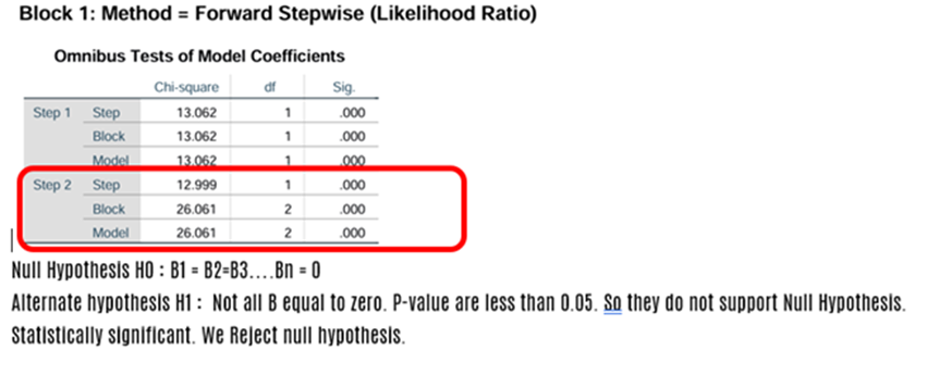
We used Forward Step-wise Likelihood Ratio method

Wald Calculation:

Age, annual salary are statistically significant as the p value of age (0.001) and annual salary (0.003) are less than 0.05.

Confidence interval at 95% for Exp(Beta) should not contain 1. For significant variable CI will not contain 1. They will be less than 1 both upper and lower. It means there is no significant relationship between age, annual salary and purchased
2. Omnibus Test: This is similar to F-Test
3.Hosmer-Lemeshow Test:(Goodness of fit test)
This is the test for finding overall fitness of the model of binary logistic regression. This is similar to Chi-Square goodness of fit test.The observations are grouped into 10 groups based on their predicted probabilities.Test is given by

Measuring the accuracy of the model
Using Classification table, you may be able to find out a) sensitivity, b) specificity, and c) ROC (Receiving Operators Characteristics). These are the important measures in the context of classification problem. Classification Table helps us to identify the accuracy of the model. Out of total purchased (Yi=1) 22, 17 (True Positive)has been correctly classified. And 5 has been taken as False Positive. Cut off value at 0.500

Cut off value : 0.300

Cut off value at 0.500
Accuracy = (TP+TN)/(TP+FP+FN+TN)
= (17+23)/(17+5+5+23)
=0.8
Precision = TP/(TP+FP)
= 17/(17+5)
=0.772727
=77.27%
Recall = TP/(TP+FN)
= 17/(17+5)
=17 / 22
=0.772727
=77.27%
Specificity = TN/(TN+FP)
= 23/(23+5)
= 23/28
=0.821429
=82.14%
When we change the cut off value to 0.300 the sensitivity and Specificity change
Sensitivity =TP/(TP+FN)
=20/20+2
=0.9090
= 90.90%
Specificity = TN/(TN+FP)
= 21/(21+7)
= 21/28
=0.75%
=82.14%

Question arises – What should be the correct cut off point?
To address this, we have to use relation concept called Receiver Operating Characteristic (ROC) curve
ROC Curve plots the true positive ratio(right positive classification) against false positive ratio(1- specificity) and compares it with random classification. The higher the area under ROC curve, the better the prediction ability. ROC plots Sensitivity on y axis and 1-specificity on x axis
Python Program