- Let (Xi, yi) be a given set of a ’n’ pairs of values X (independent variables) and Y (dependent variable)
- This is to be expressed in the form of an equation y = f(x)
- Theoretically it is useful in the study of correlation and regression.
- This enables us to represent the relationship between two variables (dependent and independent) by simple algebraic expressions.
- Expression could be Polynomial, Exponential or Logarithmic function.
- Now we can estimate the value of one variable corresponding to a specified values of other independent variables.
Linear Least Squares:
- Is the line of best fit for a group of points
- It seeks to minimize the sum of all data points of the square differences between the function value and data value.
- It is the earliest form of linear regression
- The method of least squares was first published by Legendre in 1805 and by Gauss in 1809
Fitting curve in the form of a Straight Line:
The Method of Least Squares is a procedure to determine the best fit line to data
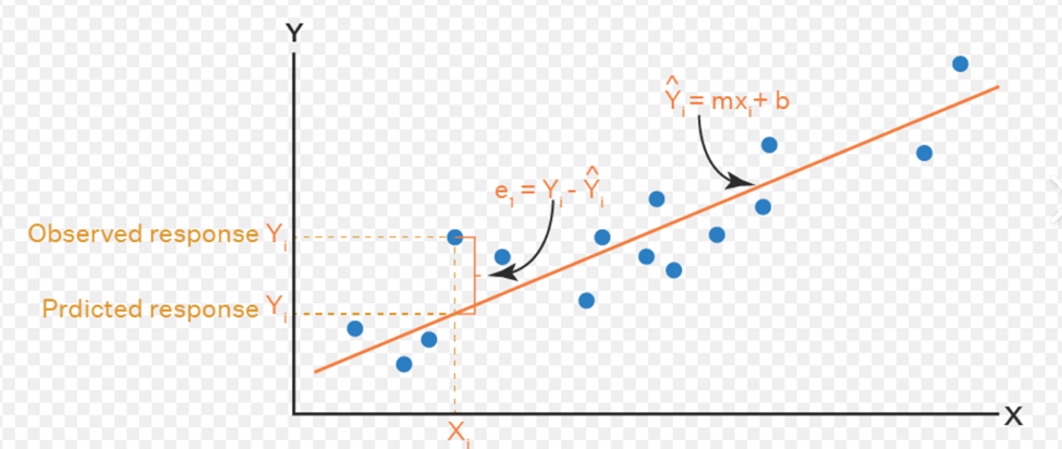
Say we plot scatter diagram for n pairs (xi, yi) We get the datapoints in the graph. When we fit it in the form of a straight line, we get an equation
Y = mx + b where m is the slope of the line and b is y intercept
The line slope could be positive (from left to right) or negative (from right to left. If it is positive, it means that y increases for every unit of change in X. If it is negative, it means that y decreases for every unit of increase in X.
For simplicity’s sake let us define the equation as y = a + bx where a is constant (y intercept) and b is the slope of the line
We have to minimize the error which is nothing but the sum of the squares of difference between the original values and the predicted values
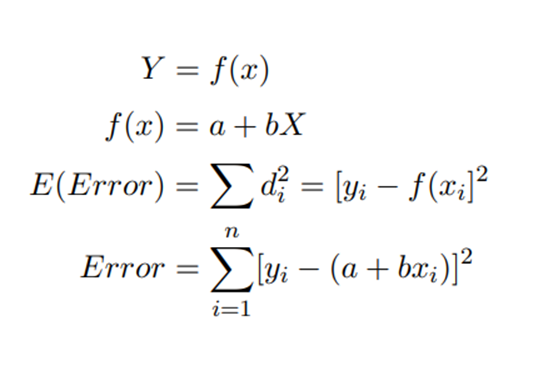
Least Square Approach:
- The ‘best’ line has minimum error between line points(predicted) and data points(observed)
- This is called the least squares approach, since square of the error is minimized
- Take the derivative of the error with respect to a and b, set each to zero.
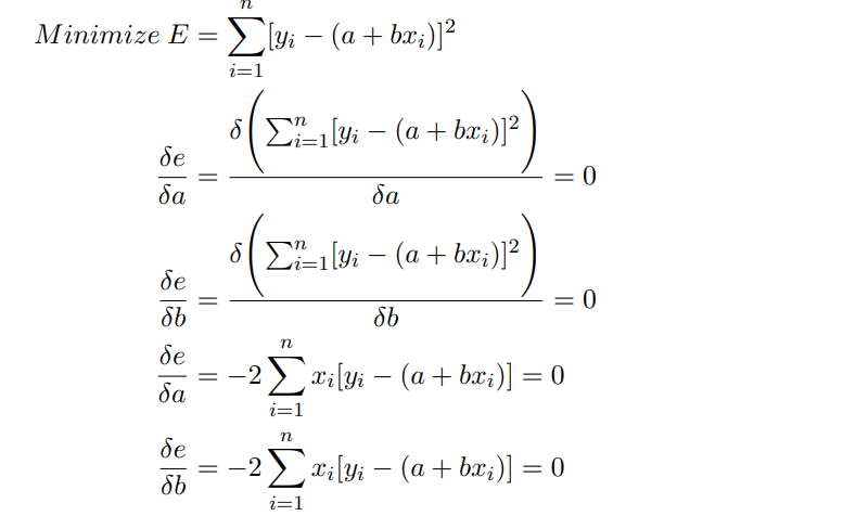
Solve for the a and b so that the previous two equations both will be equal to 0 Simplify the above and get the standard form normal equations.
Standard Normal Equation:
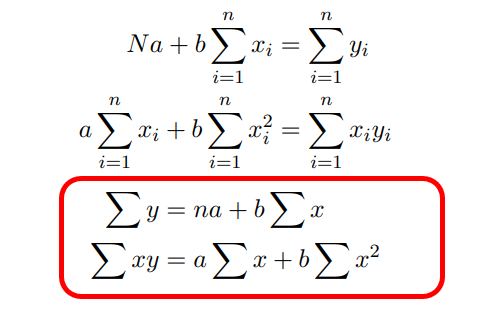
Substitute the values N, sum of Xi, sum of Yi , sum of x^2i and sum of XiYi
Using the above two equations you can find out intercept a and slope b
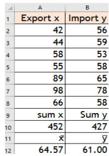
Finding a Linear Equation for the data given below:
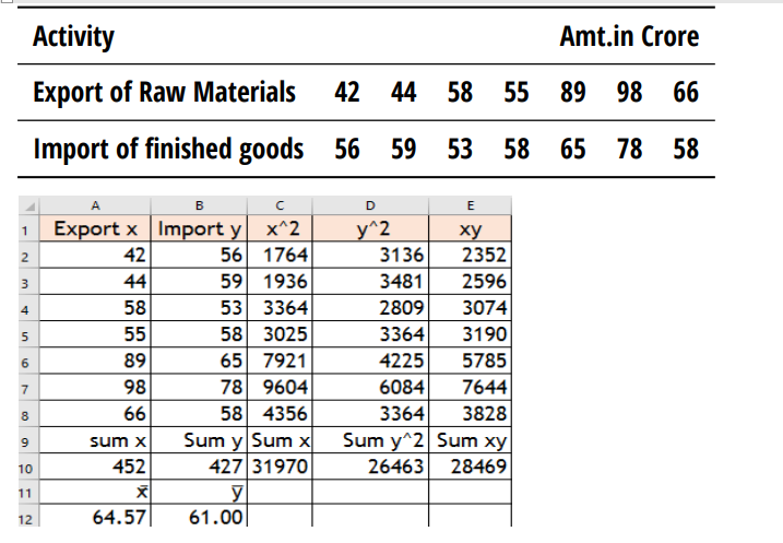
427 = 7*a + b*452 —- 1)
28469 = 452*a +31970*b —- 2)
Solve the above to fine out a and b
Multiply equation one with 452
193004 =3264*a+204304*b —- 3)
Multiply equation 2 with 7
199283=3264*a +223790*b —- 4)
Subtract 3from 4
6279= 19486*b
b(slope) =(6279/19486)
= 0.322231346
Substitute b in equation 1
427 =7a +0.322231346*452
427 = 7a +145.6486
7a = 281.3514
a(intercept) =40.19306
Equation yhat = 40.19306+0.322231346*x
Find out yhat when x = 60
Yhat = 40.19306+0.322231346*60
=40.19306+19.33388073
= 59.52694073
Solving using Excel: Same problem
Descriptive Statistics -Using Excel

Regression:

Equation arrived at:
yhat = 40.1930617 +0.32223135*x

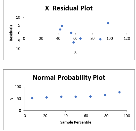
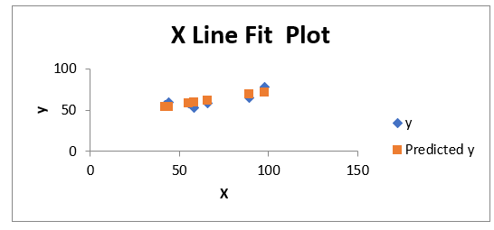
Excel Plots: