
INTRODUCTION – REGRESSION
Let us learn
- How to Construct and interpret a scatter diagram for two variables (SLR) (one dependent and one independent variable) or two or more variables (MLR) (one dependent and more than one independent variables)
- Learn the way how a scatter diagram explains the relationship between variables
- The way how a scatter diagram uses least squares to fit the best line
- The terminology used in Simple Linear Regression model
- The way how to make assumptions for that model
- The way to Determine the least squares regression
- The way how to arrive at point and interval estimates for the dependent/response variables
- The way to Determine the value of coefficient of correlation and interpret
- The way to Describe the meaning of coefficient of determination Construct confidence intervals
- The way how to Carry out Hypothesis testing for the slope of regression line Test the significance of correlation coefficient
- The way how to Examine the appropriateness of linear regression model using residual analysis.
- Certify the degree to which your underlying assumptions are met
Regression:
- The concept of regression was given by Sir Francis Galton.
- Regression is a statistical measure
- used in finance, investing and other disciplines that attempts to determine the strength of the relationship between one dependent variable (usually denoted by Y) and a series of other changing variables (known as independent variables).
- Correlation Coefficient enables us to find out the relationship between two variables using scatter diagram
- Now we try to draw a line which best represent the points
- To fit the data the line must pass close to all points and should have points on both sides.
- For this we use the technique of Least Squares
- Using the Regression, we try to quantify the dependence of one variable on the other. Say X and Y are variables. Y depends on X then the dependence is expressed in the form of equations.
We deal with two types of Variables. One is dependent variable and others are independent variables. We call these variable using different names.

We come across the following types of Regression.
- Linear Regression
- Lasso Regression
- Ridge Regression
- Polynomial regression
- Logistic Regression
- Decision Tree Regression
- Random Forest Regression
- Gradient Boosting Regression
- XGBoosting Regression
- Bagging Regression
- K-Nearest Neighbour Regression
- Catboost Regression
- Support Vector Regression
Usages of Regression Models:
Regression models are used in different functional areas of business management.
Finance:
- The capital asset pricing model (CAPM) is an often-used regression model in finance for pricing assets and discovering costs of capital.
- Probability of an account becoming NPA
- Probability of Default
- Probability of bankruptcy
- Credit Risk
Marketing:
- Prediction of Sales in the next three months based on past sales
- Prediction of market share of a company
- Prediction of customer satisfaction
- Prediction of customer churn
- Prediction of customer life time value
Operation:
- Inventory management : prediction of inventory requirement
- Productivity prediction
- Prediction of Efficiency
Human Resources:
- Prediction of Job Satisfaction among employees
- prediction of attrition
- Probability of an employee likely to go out of the company
Difference between Mathematical and Statisical Relationships:

General form of regression equation:
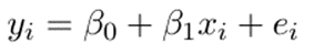
For our convenience let us use ‘a’ for intercept instead of beta not and ‘b’ for slope instead of beta one and u for regression residual instead of e

Where:
Y = the variable that you are trying to predict (dependent variable)
X = the variable that you are using to predict Y (independent variable)
a = the intercept
b = the slope
u = the regression residual
Using Regression, we try to find out a mathematical relationship between dependent and independent random variables. The relationship is in the form of a straight line(linear) that becomes the best approximate for all individual data points. Under Simple Linear Regression we use one dependent variable and one independent variable. Example Salary as independent variable and happiness as dependent variable. Under this we have Univariate data for analysis. Under Multiple Linear Regression we use one dependent variable and more than one independent variables for analysis.
Regression lines:
For a set of paired observations (Say X, Y. Y is dependent random variable and X is independent Variable) we get two straight equations.
The line is drawn in such a way that
- a) The sum of the vertical deviation is zero
- b) The sum of their squares is minimum.
Two lines
- a) Regression line of y on x. Using this you can estimate the value of Y for a given X
- b) Regression line of x on y. Using this you can estimate the value of X for a given Y
- c) The smaller the angle between these lines, the higher is the correlation between the variables
Regression Equations:
Regression Equation of Y on X

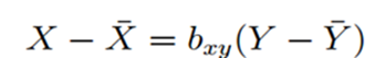
Regression Equation of X on Y
Where:
Y is the observed value (Dependent variable)
Ybar is the mean of Y
X is the observed value (independent variable)
Xbar is the mean of X
byx the regression coefficient for the line Y on X
bxy is the regression coefficient for the line X on Y
Regression line of y on x:
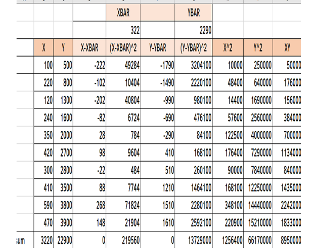
Employment and output of 10 companies are given below. You need to find out regression line using Output as dependent variable and Employment as independent variable. Employment is represented by X and output is represented by Y. Fit the regression lines using Least Square Method

Statistics – Using Least Square Method:
Let y= a+bx be the regression line of Y on X. The constants a and b can be found out using the following normal equations.


For estimating y when x=600 we use regression line of y on x

Thus, you can estimate the value dependent variable when you know the value of X
Excel


Regression Line of X on Y:
Let x= a+by be the regression line of x on y. The constants a and b can be found out using the following normal equations.


Regression Equations:
Regression Equation of Y on X
Regression Equation of X on Y
Where:
Y is the observed value (Dependent variable)
Ybar is the mean of Y
X is the observed value (independent variable)
Xbar is the mean of X
byx is the regression coefficient for the line Y on X
bxy is the regression coefficient for the line X on Y
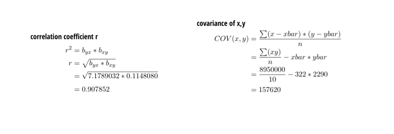
Calculation of regression Coefficients:
Correlation

Regression Coefficient for Regression Line of Y on X : byx

Regression Coefficient for Regression Line of X on Y: bxy

byx and bxy are called regression coefficients
Characteristics of Regression Coefficients:

Regression Coefficient is an absolute
- When regression is linear, then regression coefficient is given by the slope of the regression line.
- The geometric mean of regression coefficients gives the correlation coefficient (r)
measure If byx is negative then ’bxy’ is also negative and ’r’ is also negative

Formula used:


Standard error of the estimate:
- Now We can measure the strength of relationship between two variables
- We can estimate the value of one variable when we know the value of other variable
- Our estimation is based on the line of best fit.
- However some error may creep in
- Standard Error of Estimate is a measure which points out the error.
- A small Se indicates that our estimate is accurate
- Confidence level 68% when actual value of y falls between ybar- Se and ybar+Se
- Confidence level 95% can be achieved when the value of y falls between ybar-2Se and ybar+2Se
- Confidence level 99.7% can be achieved when the value of y falls between ybar-3Se and ybar+3Se

Check Standard Error:
In the previous example we found out

Result and Conclusion:
We had estimated the value of y as 3567.84 when x=500
- Se works out to 549.27
- The actual of y may lie between 3567.84-549.27 = 3018.57 and 3567.84+549.27=4117.11 when x=500
- At 95%level confidence interval would be (3018.57,4117.11)
Calculation of coefficient of determination R-Squared:
It is a measure that provides info about the goodness of fit of a model. When we talk about regression, we talk about R^2. It is a statistical measure discloses how well the regression line approximate the actual data. When a statistical model is used to predict future outcomes/in the testing of hypothesis we use the measure R^2.We use the following three sum of square metrics.


Coefficient of determination R^2 enables you to determine the goodness of fit. It is measured in percentage. Takes a value from 0 to 1. The chosen model explains 82.42% of changes of y for every one unit of change in x. Slope (b) reflects the change in y for a unit change in x
Adjusted R-Squared:
R-squared will always increase when a new predictor variable is added to the regression model. This is a drawback. Adjusted R^2 is a modified version of R^2. It adjusts the number of predictors in regression model.Adjusted R2 is a modified version of R^2
