Using IBM SPSS

Data View

Variable View
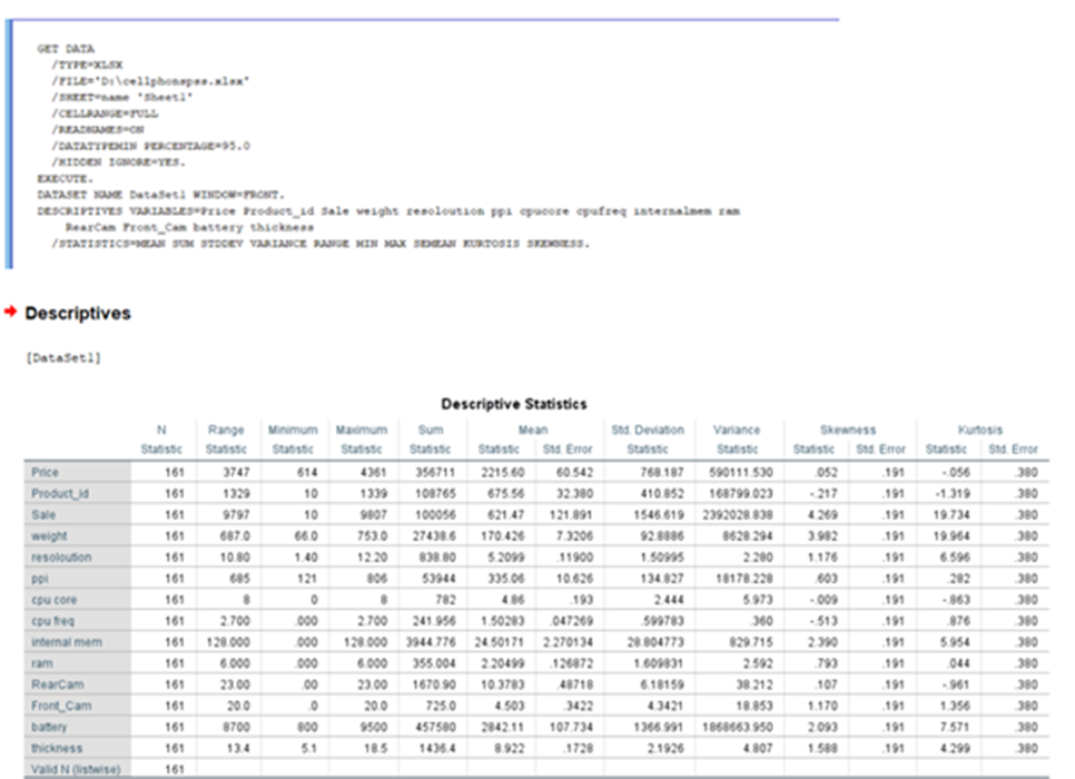
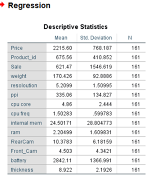
Descriptive Statistics
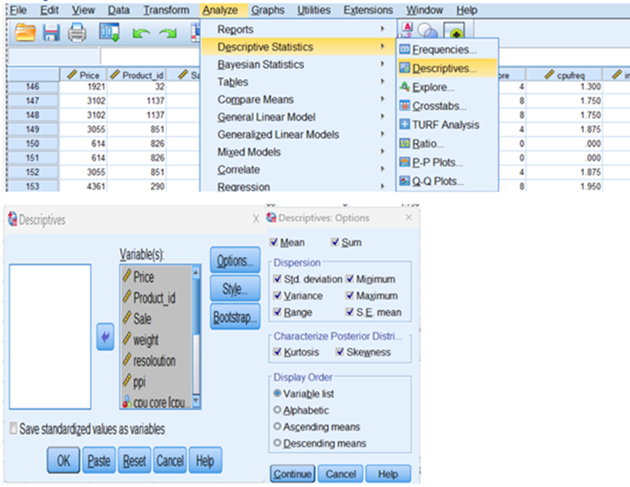
Press continue and press OK
Output in viewer
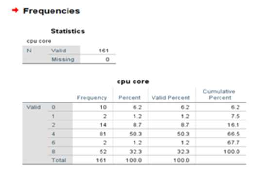
No of cpu processors used in cell phone: frequency
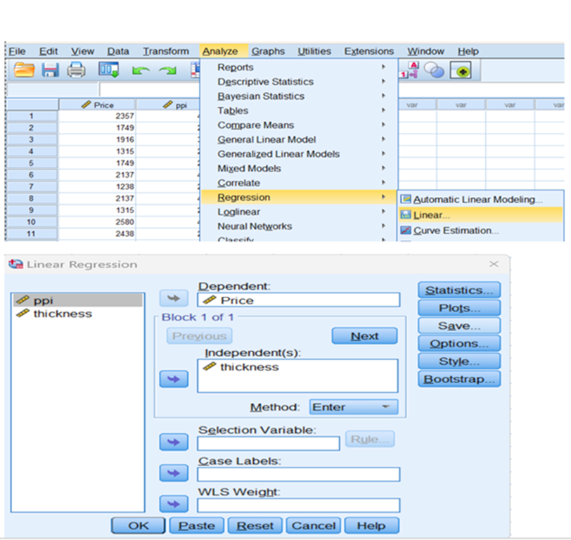
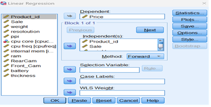
Regression
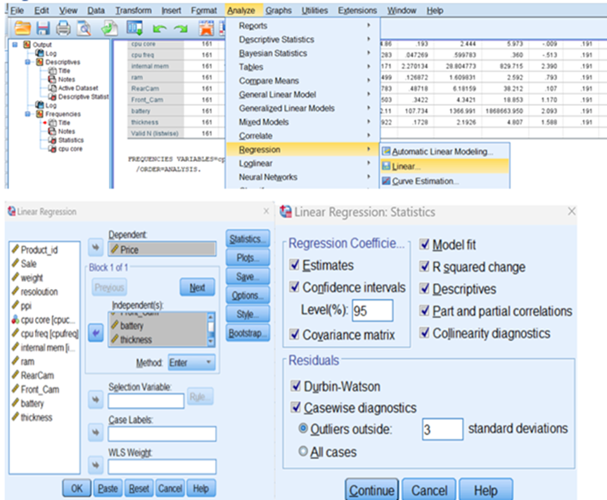
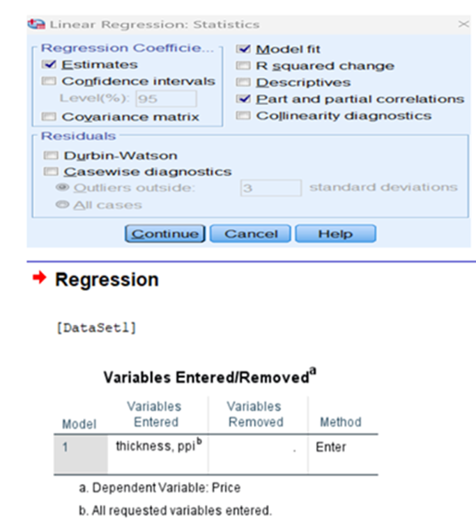
Press statistics button and fill up the popup and press continue. Then press plots button
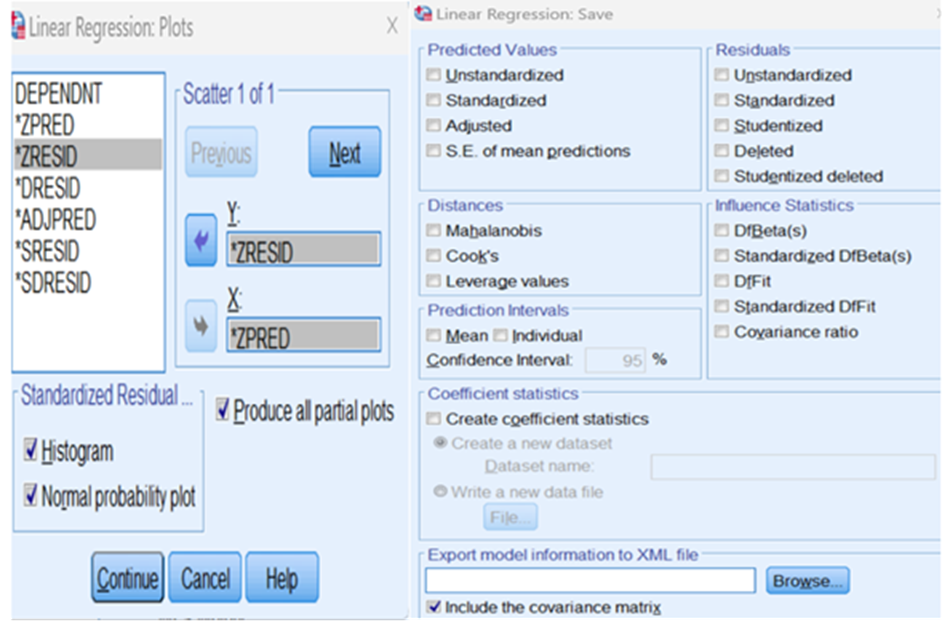
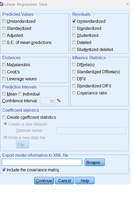
Press continue and press save button. I do not want to save anything continue and press options button
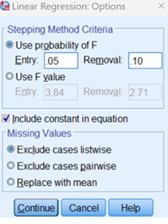
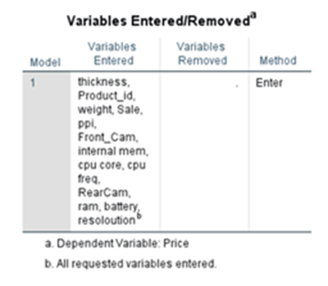
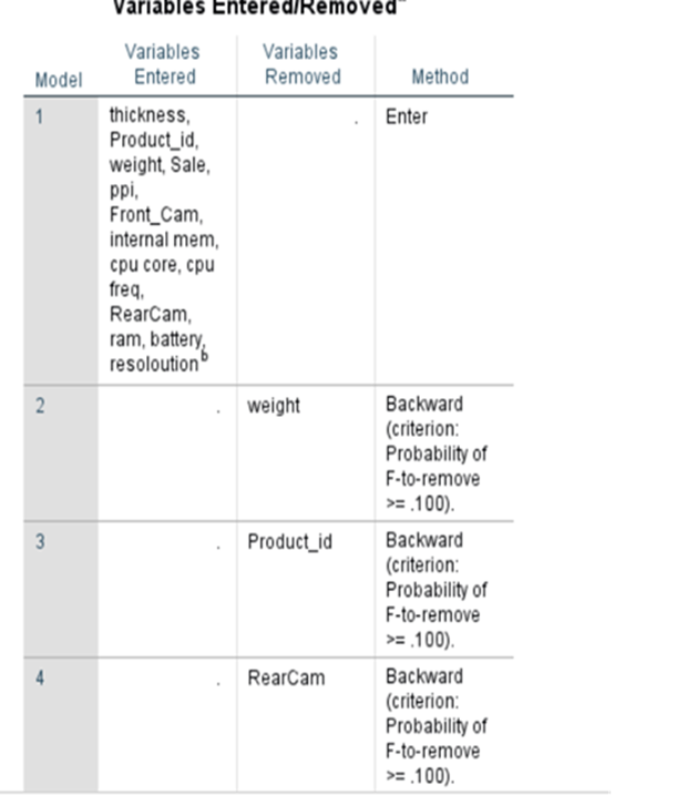
Instruct the system to enter variables if the probability falls below 0.05 and to remove the variables when the probability moves more than 0.10. Now press continue and press ok. We estimate the parameters 0, 1, 2, 3.. k using least square approach. Minimize the sum of squared errors. If we have K parameters or regression parameters in the model then we will have K+1 equations. Once we estimate regression parameters, we have to validate the model before we use. Let us imagine that we have included fourteen parameters like Price, Product_id, Sale, weight, resoloution, ppi, cpu core, cpu freq, internal mem, ram, RearCam, Front_Cam, battery, thickness in the model. We have to find out Total Cost Treatment.Say. Price is dependent/response variable and all others are explanatory variables.
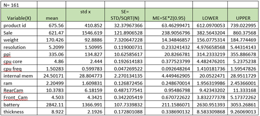
Mean and Standard Deviation of each variables:
95% Confidential Interval for mean
The population mean may fall in the range / in between Lower and Upper at (95% confidential interval)
For this we need to know mean of X, Standard Deviation of X( for each variable/feature)
- Calculate SEmean = Standard Deviation/Sqrt(n) – where n is the number of observations of sample
- Product Id SEmean = 410.852/Sqrt(161) = 37967366
- Calculate MEmean = SEmean*Zvalue (0.95) – here Z value for 95% is 1.96
- Product ID MEmean = 37967366*1.96 =63.46299471
- LCD = mean -46299471 =675.56-63.46299471 = 612.0970053
- UCD= mean+46299471= 675.56+63.46299471=739.022995
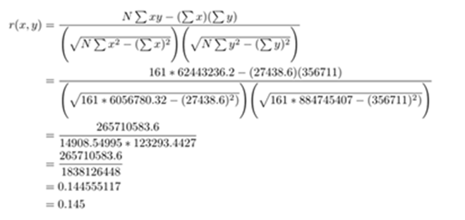
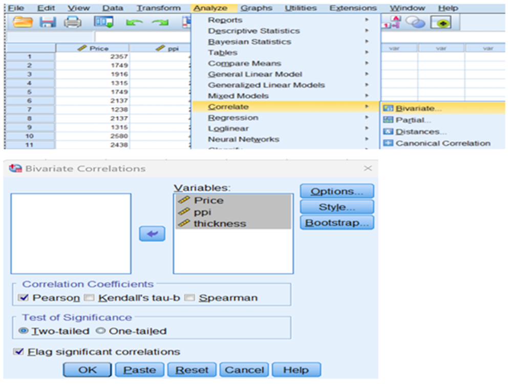
Correlation:
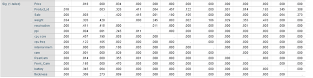
p_value using one tailed test:
Method Used: Enter
Under this method all variables whatever we provide have been entered for analysis. This is a forced inclusion of all variables in the dataset
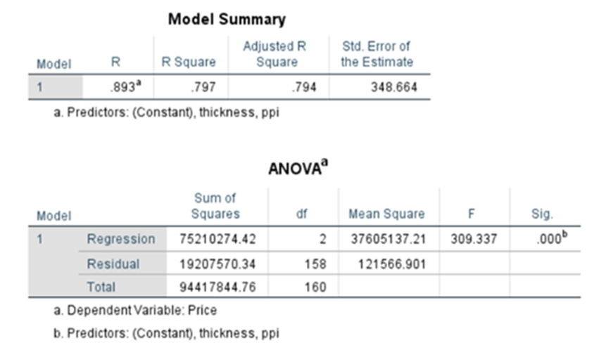
Model Summary
R is equivalent to the Pearson correlation coefficient for a simple linear regression, that is a regression with only one predictor variable.
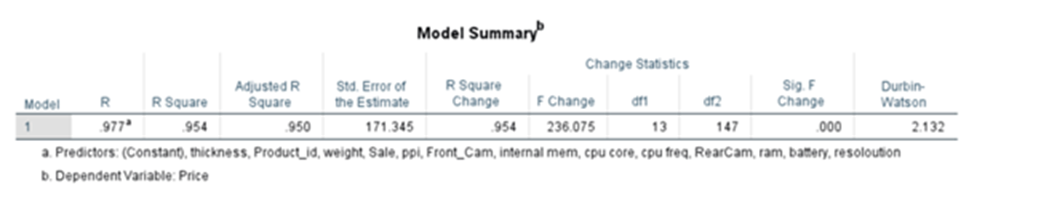
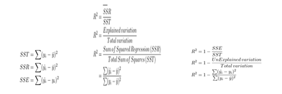
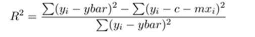
Coefficient of Determination –> R^2(R-SQUARE)
R2 comes to 0.954,namely, 95.4% of changes in dependent variable price is explained by the unit change of each independent variable. Besides that, adjusted R2 is calculated as 0.950 i.e. 95%. At the time of adding a new independent variable for consideration, R2 increases. This may be due to multi-collinearity. To avoid that Adjusted R^2 was introduced.
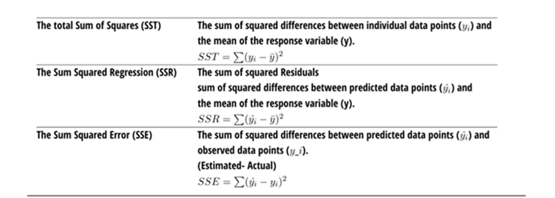
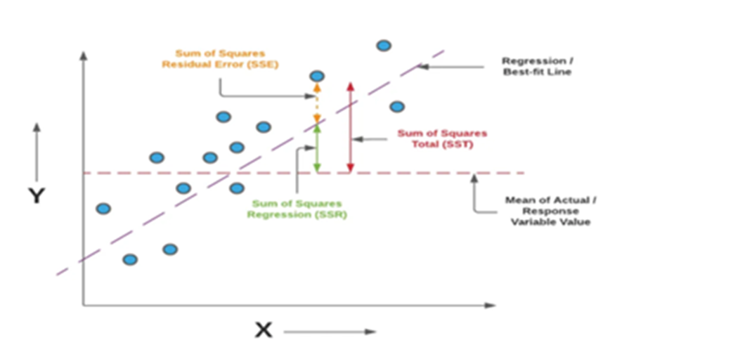
It is a measure that provides info about the goodness of fit of a model. When we talk about regression, we talk about R^2. It is a statistical measure that discloses how well the regression line approximates the actual data. When a statistical model is used to predict future outcomes/ in the testing of hypothesis we use this measure R^2, an important measure. We use the following three sum of squares metric
Formulae
Example:
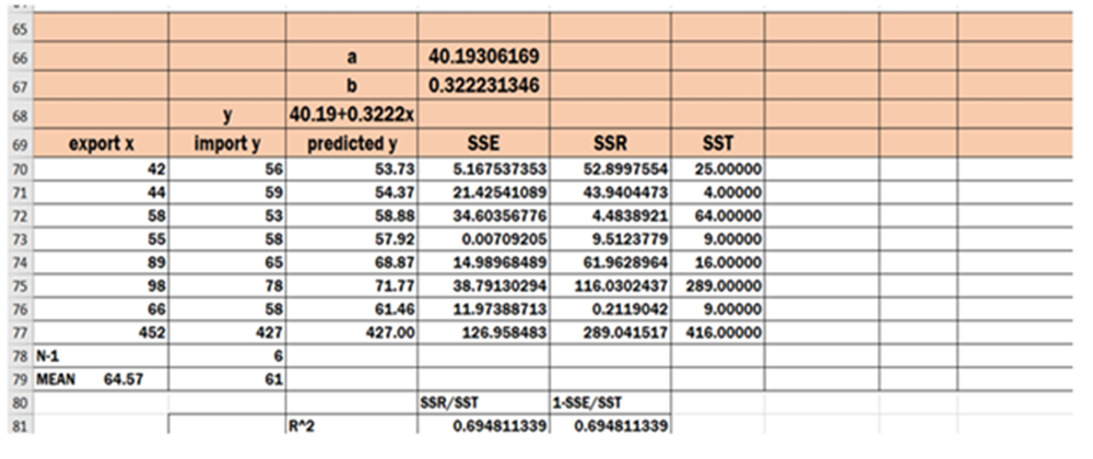
Find mean for export(X) – 452/7 = 64.57
find mean for import (y). – 427/7 = 61.00
No.of observations are 7 .
Find predicted y using the formula 40.19+0.3222x for each individual value of X.
Find SSE(Sum of Squares of Error) using formula SSE = SUM(yhat- y)^2=126.96
Find SSR(Sum of Squares of Residuals) using formula SSR=SUM(yhat-mean(y))^2 =289.04
Find SST(Total Sum of Squares) using formula SST= SUM(y- mean(y))^2 = 416.00
RSquare = SSR/SST = 289.04/416 =0.6948 = 69.48%
RSquare = 1-(SSE/SST) = 1-(126.96/416.00) = 0.6948 = 69.48%
The above said example is taken from Simple Linear Regression model. Coefficient of determination R^2 enables you to determine the goodness of fit. It is measured in percentage. Takes a value from 0 to 1. The chosen model explains 69.48 % of changes of y for every one unit of change in x. Slope (b) reflects the change in y for a unit change in X
Multiple R-Square
This is meant for multiple linear regression
R-square shows the total variation for the dependent variable that could be explained by the independent variables. A value greater than 0.5 shows that the model is effective enough to determine the relationship. In this case, the value is .6948, which is good.
R-Correlation
R = SQRT(R^2)
= SQRT(0.954)
=0.977
R-value represents the correlation between the dependent and independent variableW. A value greater than 0.4 is taken for further analysis. In this case, the value is .977, which is good.
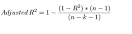
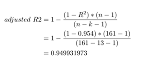
Adjusted R-Square
R-squared will always increase when a new predictor variable is added to the regression model. This is a drawback. Adjusted R^2 is a modified version of R^2. It adjusts the number of predictors in regression model Adjusted R^2 is a modified version of R^2 Calculated as under:
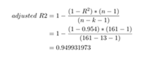
Adjusted R-square shows the generalization of the results i.e. the variation of the sample results from the population in multiple regression. The difference between R-square and Adjusted R-square should be minimum. In this case, the value is .950, which is not far off from .954, so it is good. Therefore, the model summary table is satisfactory to proceed with the next step
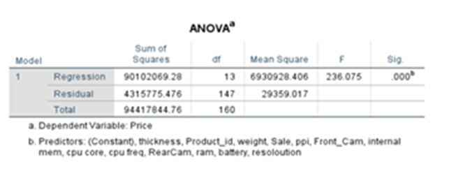
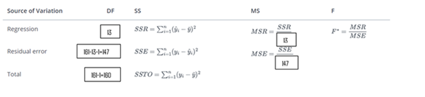
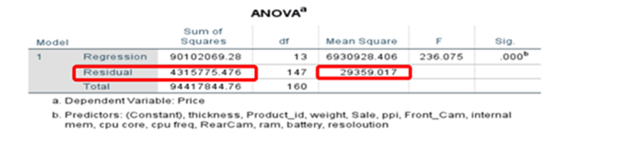
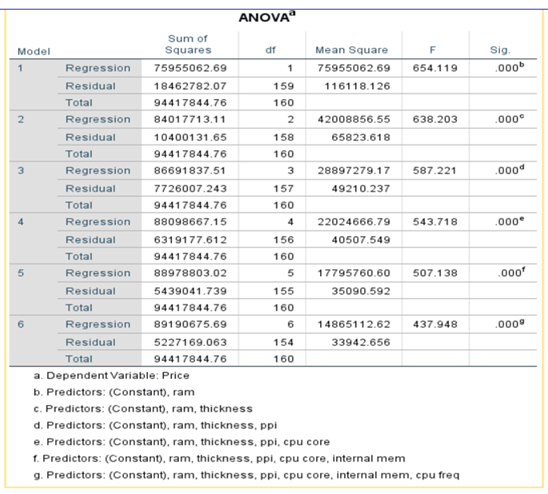
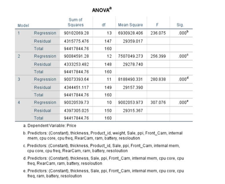
ANOVA TABLE
It determines whether the model is significant enough to determine the outcome.
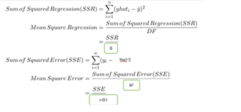
Sum of Squares of Regression(SSR) =∑(yhat – ybar)^2 = 90102069.28
Sum of squares of Residual(SSR/SSE) = ∑(y – yhat)^2 = 4315775.476
Sum of squares of Total = ∑(y – ybar)^2 =94417844.76
Mean Square Regression(MSR) = SSR/df = 90102069.28/13 = 6930928.406
Mean Square Error(MSE) = SSE/df = 4315775.476/147 = 29359.017
F-statistic = MSR/MSE = 6930928.406/29359.017 =236.075
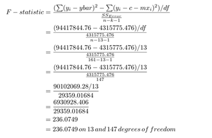
p-value of F-statistic = 0.000.
Since p-value is less than 0.05 we reject Null hypothesis and come to a conclusion the parameters are statistically significant and each one of beta is not equal to zero. F-test is passed.
P-value/ Sig value: Generally, 95% confidence interval or 5% level of the significance level is chosen for the study. The p-value should be less than 0.05. In the above table, it is .000. Therefore, the result is significant. There is a possibility of rejecting the null hypothesis. Based on the t-statistic test statistic and the degrees of freedom, we determine the P-value. P-value is the smallest for which we can reject Null H0.
F-ratio: It represents an improvement in the prediction of the variable by fitting the model after considering the inaccuracy present in the model. A value is greater than 1 for F-ratio yield efficient model. In the above table, the value is 236.05, which is good. Here the value of F is greater than 25, which is ratio of MSR over MSE and the corresponding P value is very, very low, which is basically almost close to zero. We can conclude that the overall model is statistically significant
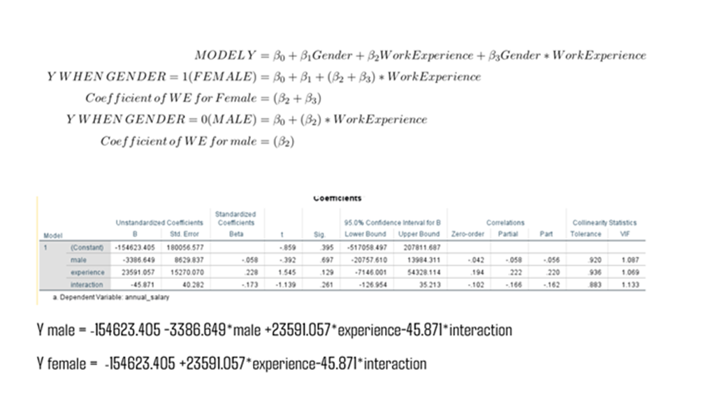
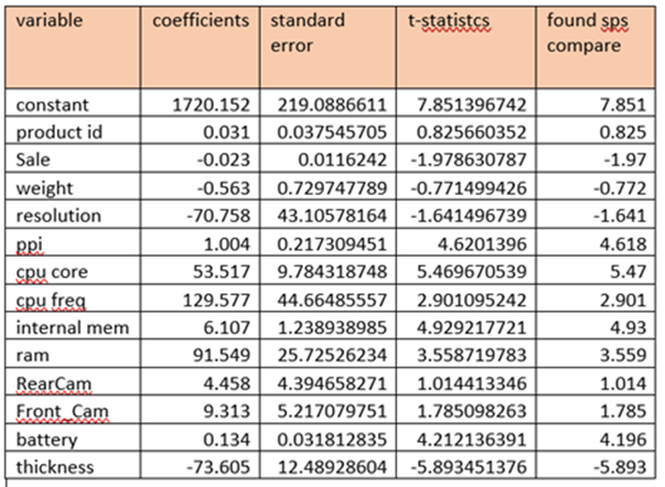
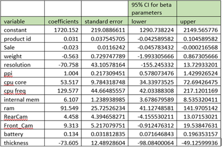
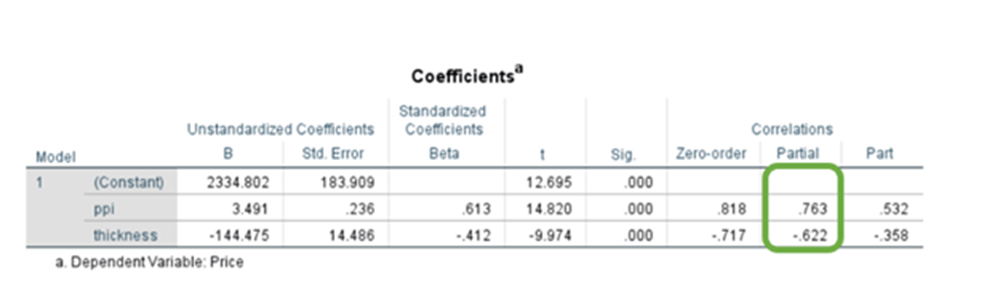
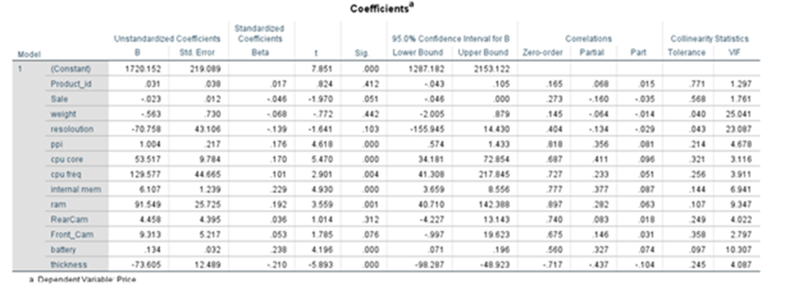
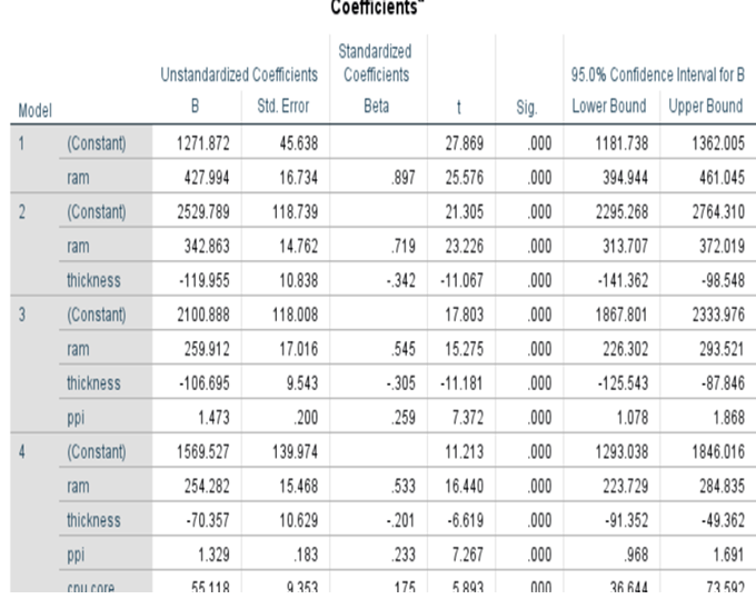
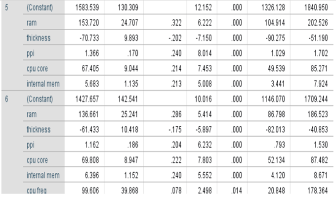
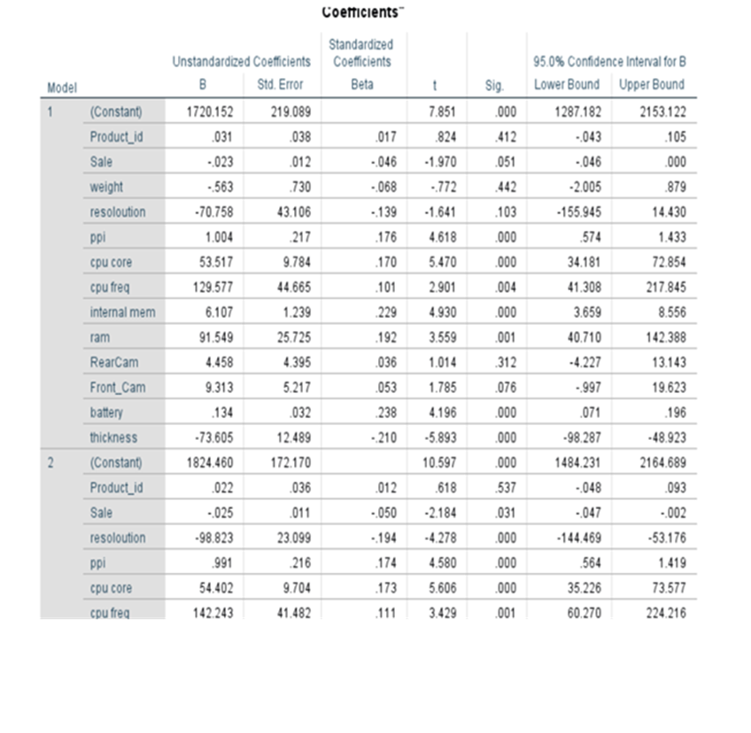
Coefficients
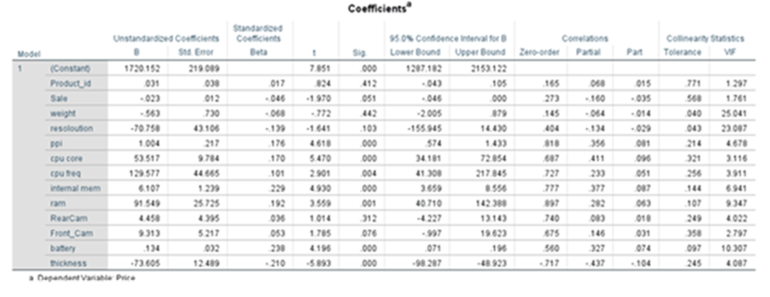
Equation of the fitted line:
Price(yhat) = 1720.152+0.031*product_id -0.023*sale -0.563*weight-70.758*resolution +1.004*ppi +53.517*cpu core +129.577*cpu freq +6.107*internal mem
+91.549*ram + 4.458*RearCam+9.313*Front_cam+1.34*battery-73.605*thickness
Shows the strength of relationship and significance of the variable in the model and shows how it impacts the dependent variable. Enables you to perform hypothesis testing for further study. Sig/p-value of parameters/coefficients of variables like product_id, sale, weight, resoloution, RearCam, and Front_Cam are greater than 0.05. These are not significant. Other seven parameters are with p-value less than 0.05.
The Sig.value should be below the tolerable level of significance for the study (0.05 or 95% Confidence level). Based on the significant value the null hypothesis is either rejected or accepted
If sig.value is <0.05 the null hypothesis is rejected. it means there is an impact
If sig.value is >0.05 the null hypothesis is accepted. There is no strong evidence to reject the Null hypothesis. it means there is no impact.
Sometimes some variables may be statistically insignificant due to multi-collinearity. We have to take care of this issue. Say the coefficient of product_id is 0.031. This is like serial numbers. It will not have any influence on the price. The coefficient of weight is -.563. It means that the price of the phone decreases by -0.563 when there is an increase of one kilo gram of body weight provided everything else is kept constant. That means we control all other variables.
Standared Errors of Coefficients/Betas
The variance of the coefficients is derived from the variance-covariance matrix of the estimated coefficients. The formula for the variance of each coefficient βj is given by:
Var(βj)=MSE⋅(X′X)−1j
Var(βj)=MSE⋅(X′X)j−1
Where:
– XX is the matrix of independent variables (including a column of ones for the intercept).
– X′Xis the matrix product of XX transposed and XX.
– (X′X)−1jj(X′X)j−1 is the j-th diagonal element of the inverse of the X′X matrix.
Calculate the standard errors of Coefficients
The standard error of each coefficient βj.
βj is the square root of its variance:
SE(βj)=√Var(βj)
Using Python Program
dfData <- as.data.frame(read.csv(“https://gattonweb.uky.edu/sheather/book/docs/datasets/MichelinNY.csv”,header=T))
# using direct calculations
vY <- as.matrix(dfData[, -2])[, 5] # dependent variable
mX <- cbind(constant = 1, as.matrix(dfData[, -2])[, -5]) # design matrix
vBeta <- solve(t(mX)%*%mX, t(mX)%*%vY) # coefficient estimates
dSigmaSq <- sum((vY – mX%*%vBeta)^2)/(nrow(mX)-ncol(mX)) # estimate of sigma-squared
mVarCovar <- dSigmaSq*chol2inv(chol(t(mX)%*%mX)) # variance covariance matrix
vStdErr <- sqrt(diag(mVarCovar)) # coeff. est. standard errors
print(cbind(vBeta, vStdErr)) # output
Using statsmodels.api
model.bse
Using Excel:
Refer to Excel section topic Calculation of Standard Error of all Betas:
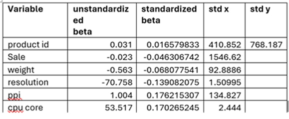
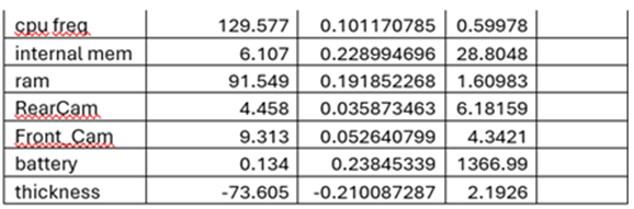
Standardized Betas
When we deal with multiple variables measured in different units (say body weight in kg, body height in cm etc we cannot compare them. In order to standardize response variable, we have to standardize all explanatory variables. After standardization, we get standard beta coefficients. The variable which has the highest standardized beta coefficient will have the maximum influence on Response variable.
Standardized Beta is nothing but the raw beta that we get times standard deviation of that explanatory variable over standard deviation of Y
Standardize Beta = (Unstandardized Beta * standard deviation of X)/standard deviation of y
t-Statistics calculation
t-statistics = Coefficients(beta)/Standard Error(beta)
p_value statistics
It can be calculated on web using p-value calculator
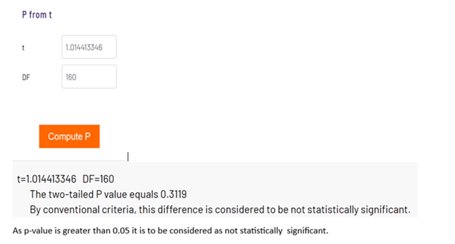
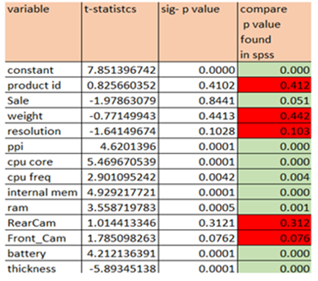
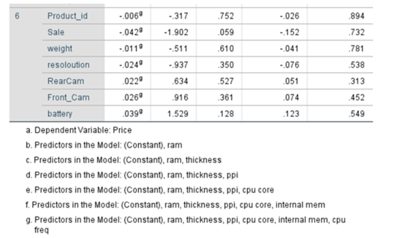
The p-values related to product_id, weight, resoloution, RearCam and Front_Cam are greater than 0.05 these variables can be removed from regression line findings provided these are not influenced by multi collinearity.
Using t-Distribution Table
You can find p-value using t-Distribution value. Here look up for degrees of freedom. We have 161 observations. And Degrees of Freedom is 161-1 = 160
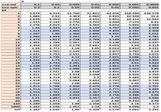
Remember the drawback of using the t distribution table: it does not tell us the exact p-value; it only gives us a range of values.
95% Confidential Interval of beta
Lower bound and Upper bound
Lower bound = coefficient(beta) – 1.96*standard error(beta)
Upper bound = coefficient(beta) + 1.96*Standard error(beta)
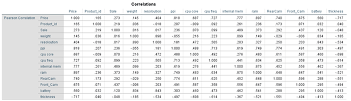
Correlations
To determine the relation between two variables we use different types of correlations
- Pearson Correlation
- Spearman Correlation
- Point Biserial Correlation
- Kendall Correlation
And the terms we come across are
- Zero-order Correlation
- Partial Correlation
- Part Correlation
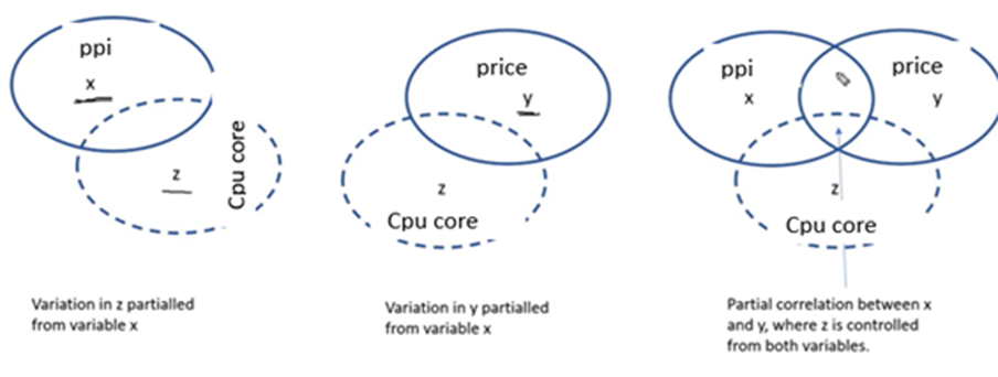
These types of correlations are required/relevant when you have response/dependent variable(aka outcome variable) predictor/independent variables (aka explanatory variables) One or more control variables(confounding variables)
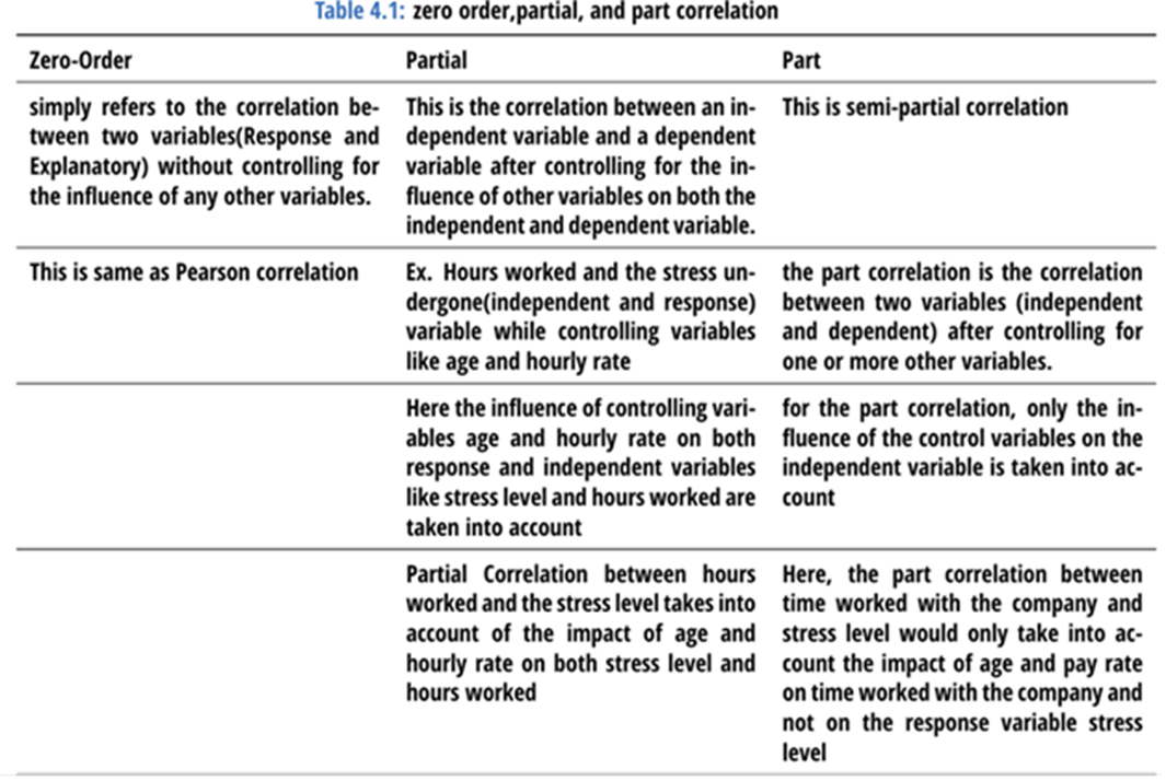
Partial Correlation and Part correlation provides another means of assessing the relative importance of independent variables in determining the value of y ( response variable). They show how much each variable uniquely contributes to R^2.
Partial Correlation: Describes how each independent variables participation in determining partial correlation pr and its square pr^2. Squared pr^2 explains “How much of the Y variance which is not estimated by the other independent variables in the equation is estimated by this variable?”
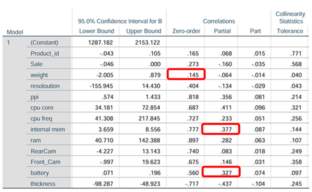
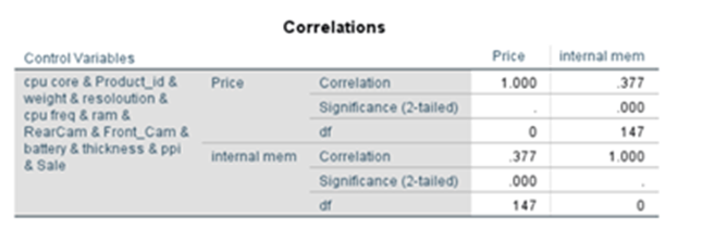
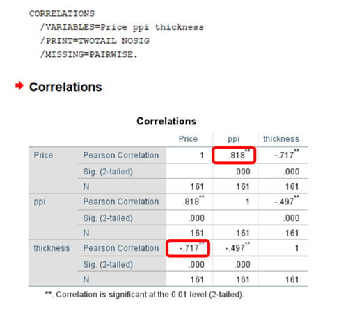
Zero order correlation is nothing but Pearson correlation. You can compute Pearson correlation between each feature with dependent variable Price(y)
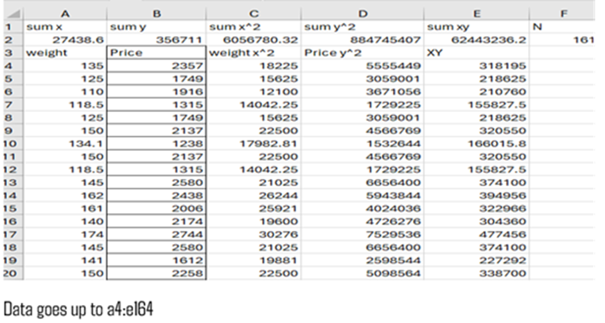
Let us find out the correlation r(weight,price)
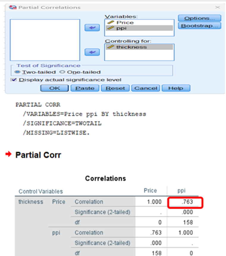
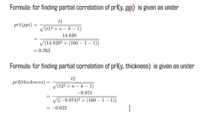
Calculation of Partial Correlation:
Calculates the correlation between two variables, while excluding the effect of a third variable.
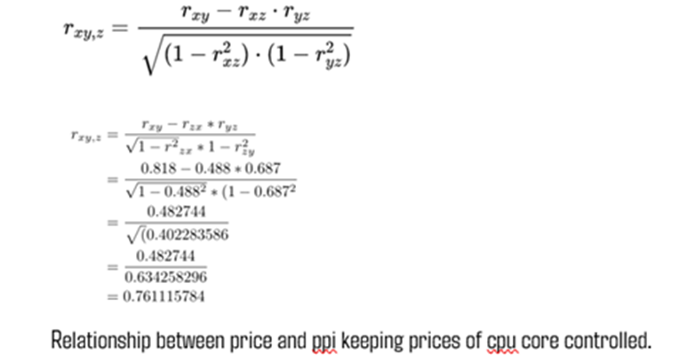
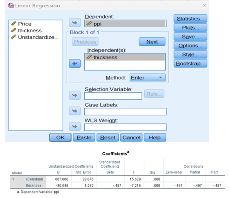
Let us take the Pearson correlation between y and ppi and y and cpu core
r(ppi, price (xy) ) = 0.818
r(cpu core, price (zy)=0.687
r(cpu core, ppi (zx) =0.488
Controlling variable z. our aim is to find out correlation rxy,z
The partial correlation rxy,z tells how strongly the variable x correlates with the variable y, if the correlation of both variables with the variable z is calculated out.
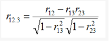
Formula
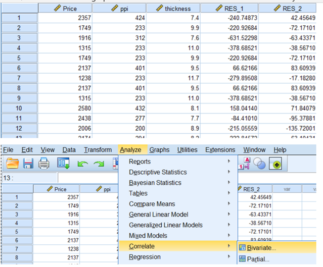
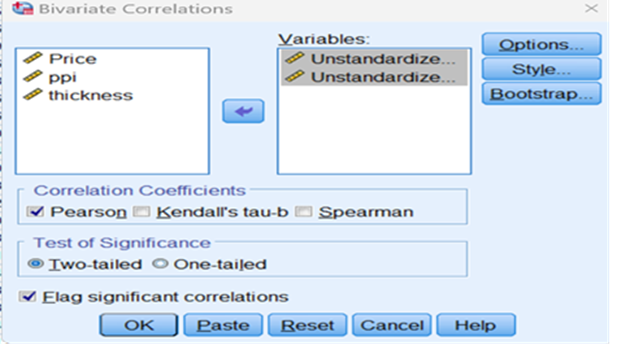
Can be done using SPSS
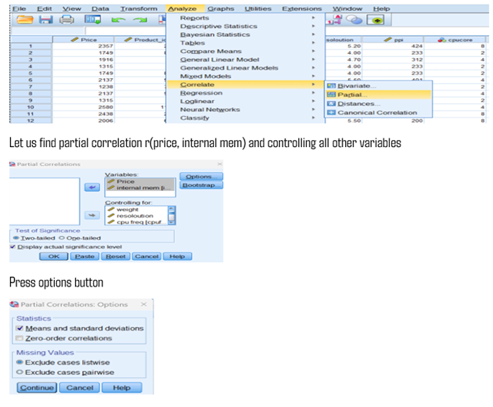
If you need Zero-order correlation you can tick mark. Otherwise continue
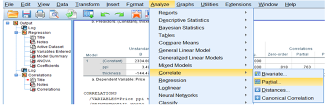
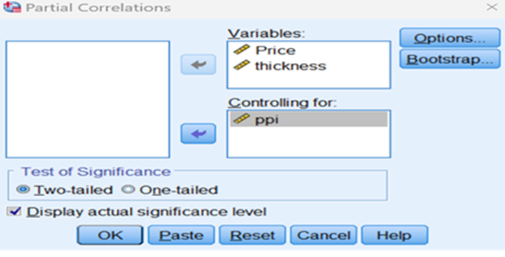
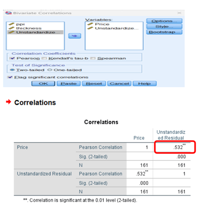
Now we can find partial correlation between (price, battery) and controlling all other variables
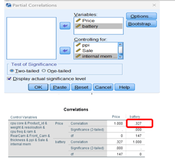
In the same way you can find partial correlation between price and required feature subject to controlling all other variables
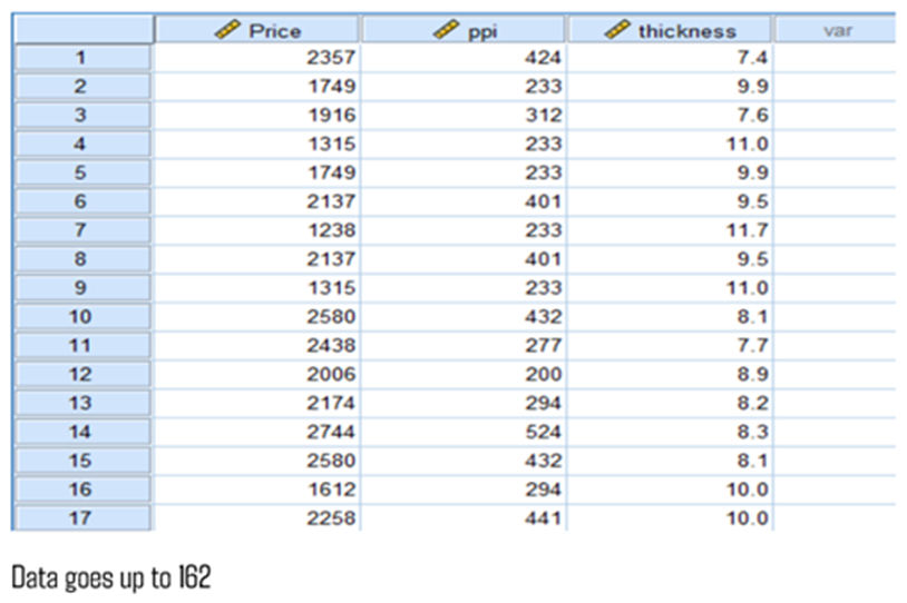
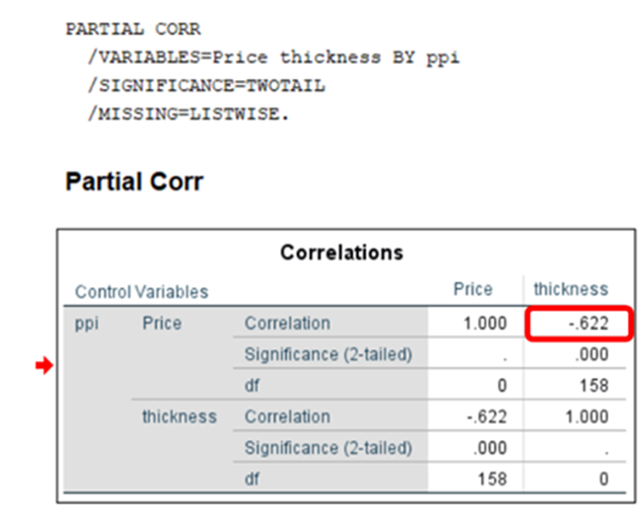
Let us restrict the above data with three features, price(y) and ppi and thickness (independent variables)
correlation bivariate
Partial correlation
Part Correlation:
Part correlation is similar to partial correlation. But there is a subtle difference.
Sometimes, it is called Semi-Correlation.
Like the partial correlation, the part correlation is the correlation between two variables (independent and dependent) after controlling for one or more other variables.
With semi-partial correlation, the third variable holds constant for either X or Y but not both;
with partial, the third variable holds constant for both X and Y.
It explains how one specific independent variable affects the dependent variable, while other variables are controlled for to prevent them getting in the way.
However, for the part correlation, only the influence of the control variables on the independent variable is taken into account. In other words, the part correlation does not control for the influence of the confounding variables on the dependent variable.
It indicates the “unique” contribution of an independent variable. Specifically, the squared semi-partial correlation for a variable tells us how much R^2 will decrease if that variable is removed from the regression equation.
Semipartial correlation measures the strength of linear relationship between variables X1 and X2 holding X3 constant for just X1 or just X2. It is also called part correlation.
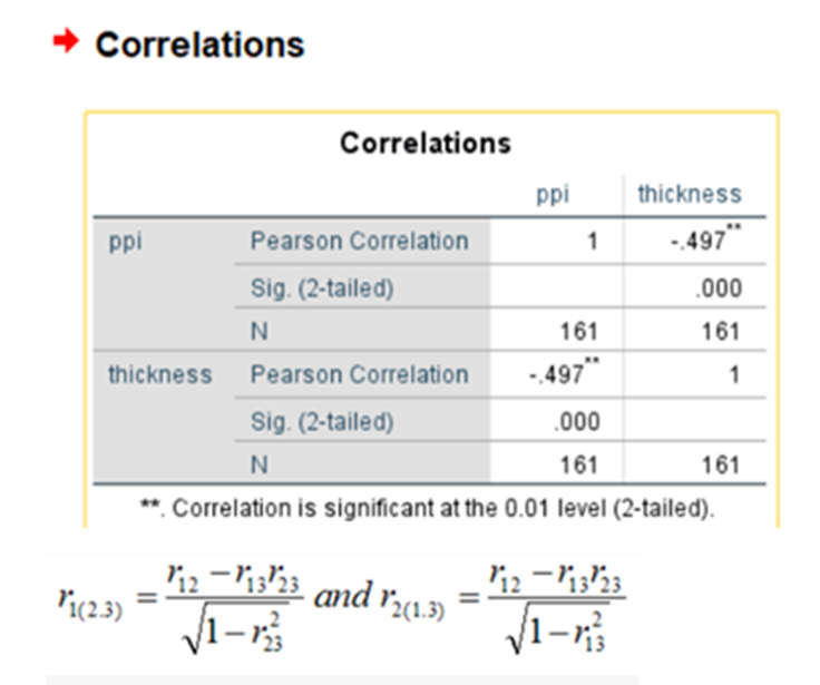
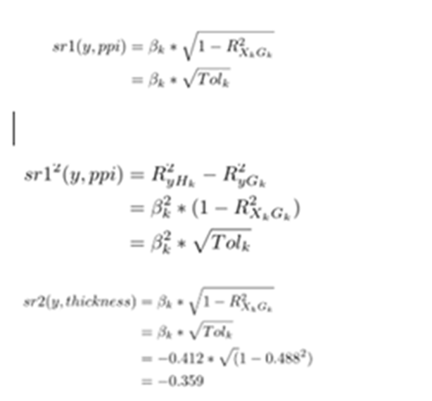
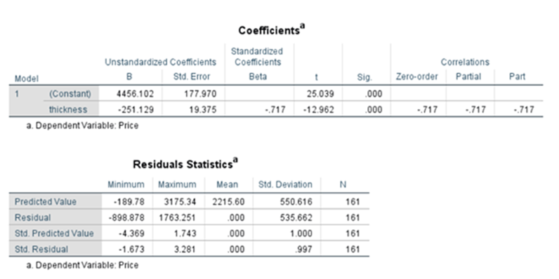
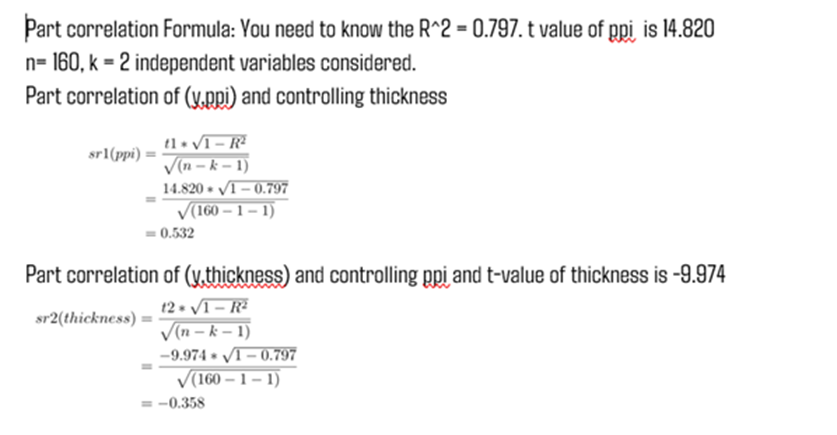
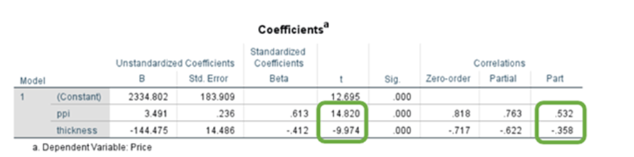
r12 =0.818 (r(price,ppi)
r13 = -0.717(r(price,thickness)
r23 =-0.497(r(ppi,thickness)
r1(2.3) = 0.818-(-0.717)*(-0.497) / sqrt(1-(-0.497)^2)
= 0.532009 relationship between price and ppi when thickness is remaining constant for ppi
In the above image, r1(2.3) means the semipartial correlation between variables X1 and X2 where X3 is constant for X2.
Multi Linear Regression Model Diagnostics
You must know how a model(formula) is validated and diagnosed
Step 1: Test for overall fitness of the model
Step 2: Test for overall model significance achieved through F-test
Step 3: Check for individual explanatory variable and their statistical significance(achieved through t-test)
Step 4: Check for multi-collinearity and auto correlation
Step 1:Test for Overall Fitness of the model
Coefficient of Determination R^2:
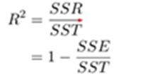
Where:
SSR = Sum of Squares of Residuals ∑(yhat-ybar)^2
SSE = Sum of Squares of Error ∑(y – yhat)^2
SST = Total Sum of Squares ∑(y – ybar)^2
SSR(Numerator) will go on increasing as the number of explanatory variables increases
SSE will go on decreasing when you add new independent variable for analysis
So as and when you add a new independent variable, R2 will increase irrespective of the matter if the added variable is statistically significant or not.
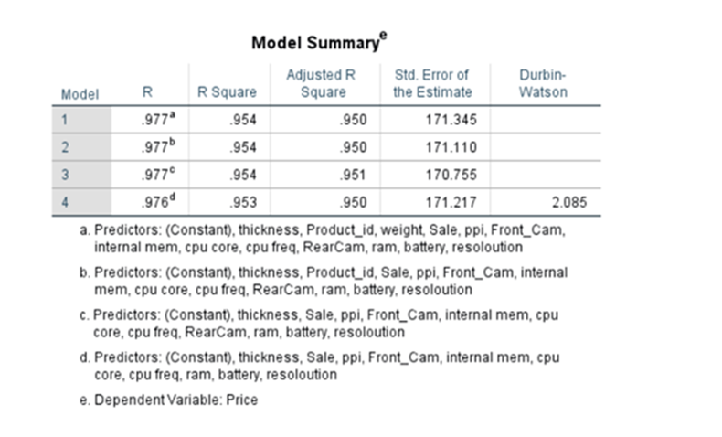
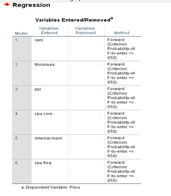
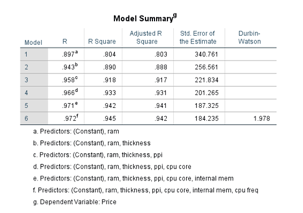
Under step-wise method see the model summary
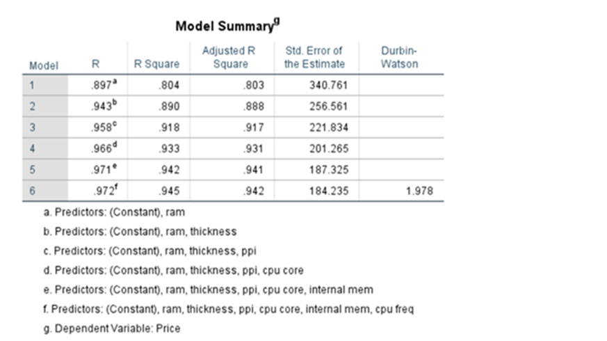
System adds or removes the features/predictor variables on condition basis and finally it settles down by adding 7 variables(including constant). When ‘ram’ was added R^2 was 0.804 when it added thickness R^2 increased to 0.890 and finally after including 7 variables R^2 increased to 0.945. But when we used Enter method where all variables 13 were added at the beginning itself. The R^2 was 0.954
To nullify the effect of increase on every addition of independent variable we have to find out Adjusted R2. Here we normalize both numerator and denominator with respect to degrees of freedom. Say n is the number of observations and k is the number of variables used in the model
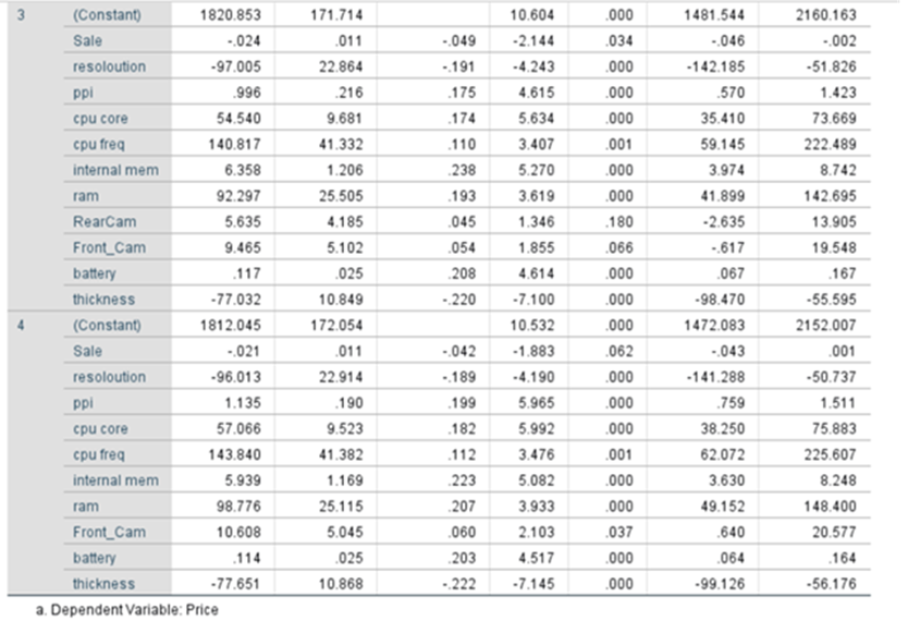
Under Enter Method: The model was
Price(yhat) = 1720.152+0.031*product_id -0.023*sale -0.563*weight-70.758*resolution
+1.004*ppi +53.517*cpu core +129.577*cpu freq +6.107*internal mem
+91.549*ram + 4.458*RearCam+9.313*Front_cam+1.34*battery-73.605*thickness
When we add a new variable R^2 will increase where as Adjusted R^2 will not increase
Step2: Test for overall model significance
It is achieved through F-test For multiple linear regression we will have more than one independent variables.
Hypothesis for F-test
Null H_0: (null hypothesis) beta_0$,beta_1,beta_2,beta_3…beta k will be equal to 0
Alternate H_1: beta_0,beta_1,beta_2,beta_3…beta k will not be equal to zero.
sometimes some betas may be zero.
If we reject Null hypothesis, it means that we can claim that overall model is valid
Remember, some explanatory variables could be statistically insignificant
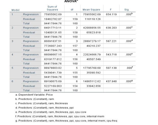
We get this ANOVA (Analysis of Variance) Table. F is related to R^2
Refer to Anova Table in the previous pages
Step 3: Check for individual explanatory variable and their statistical significance(achieved through t-test)
Here we use t-test
Null H_0: (null hypothesis) beta_0,beta_1$,beta_2,beta_3…beta k= 0
Alternate H_1: beta_0,beta_1,beta_2,beta_3…beta_k<>0
Coefficient Table
We are having 13 variables plus one constant.
p-values for all variables are less than 0.05 except for product_id, sale, weight, resoloution, RearCam, and Front_Cam. We reject the null hypothesis for the variables which have p-values less than .05. All are statistically significant. The Variables that may appear with p-value greater than 0.05 may be dropped. At the same we cannot remove beta_0 even though the p-value exceeds 0.05. It is an intercept constant. Perhaps some may have p-value greater than 0.05 due to multi collinearity,
Check for Multi-Collinearity and Auto Correlation
Multi-collinearity is a serious issue in MLR model. It is nothing but high correlation between explanatory variables. It can lead to unstable coefficients. Understand the impact multi-collinearity.
P-value of weight increases to 0.442 as we add new variables. This is higher than 0.05. weight has become statistically insignificant. This happens because of multi-collinearity we may see high R^2
F-test rejects Null Hypothesis. It means that F-test reports that overall model is fine. But none of the t-test rejects Null Hypothesis.
There is a contradiction between F-test and t-test The correlation between X variables are high compared to correlation between X and Y
Because of this regression coefficient estimates are inflated. This produces bad results when I do t-test
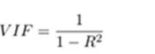
Variation Inflation Factor (VIF)
How to identify the existence of Multi-collinearity?
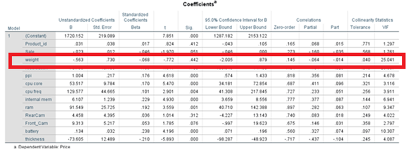
One of the measures used to identify the existence of Multi-Collinearity is Variance Inflation Factor(VIF). It is given by
Say if VIF is 25.041 then Standard Error of estimate is inflated by (sqrt(V IF) ie by 5.004098
When standard error of estimate is inflated by 5 then t-value is deflated by the factor 5.
When t-value goes down p-value increases
So you may decide to remove the variable weight thinking that the variable is significantly insignificant.
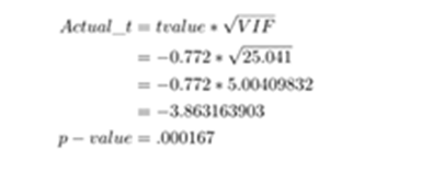
p-Value Calculation

The result is significant as p < .05. we cannot remove this variable
Now explanatory weight is significant. People may not like to remove variables. In that case we may go and use Principal Component Analysis.
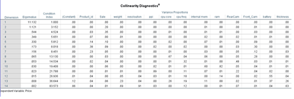
Collinearity Diagnostics
It is applicable only for Multiple Linear Regression model
Condition Index
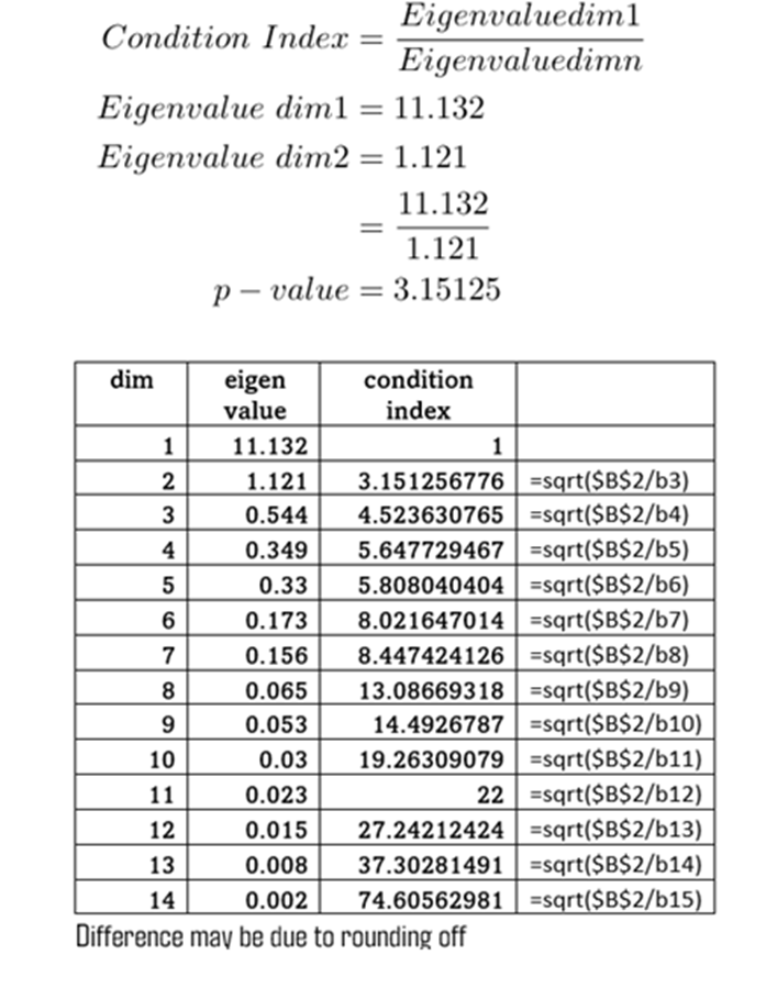
Dimension
First column talks about dimension. Then comes Eigen value and condition Index
First column dimension is similar but not identical to a factor analysis or PCA (principal component analysis)
Eigen Value
Eigenvalues close to 0 are an indication for multicollinearity. To be seen in conjunction with condition index
Condition Index
Condition index is calculated from eigen values
Condition index = Sqrt( Eigen value Dim1 /Eigen value Dim2 or Dim3…Dim n)
Interpretation of condition Index
Values above 15 indicates multi-collinearity issues.
Values above 30 indicates very strong sign of multi-collinearity problems
Variance Proportions
We also get regression coefficients variance decomposition matrix. According to Hair et al. (2013) for each row with a high Condition Index, you search for values above .90 in the Variance Proportions. If you find two or more values above .90 in one line you can assume that there is a collinearity problem between those predictors. If only one predictor in a line has a value above .90, this is not a sign for multicollinearity.
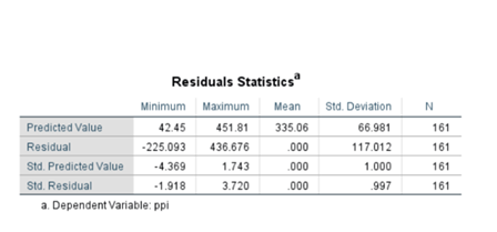
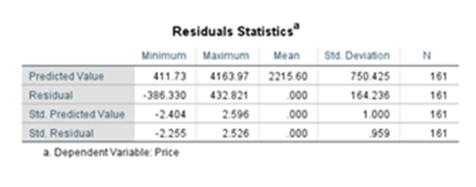
Residual Statistitcs
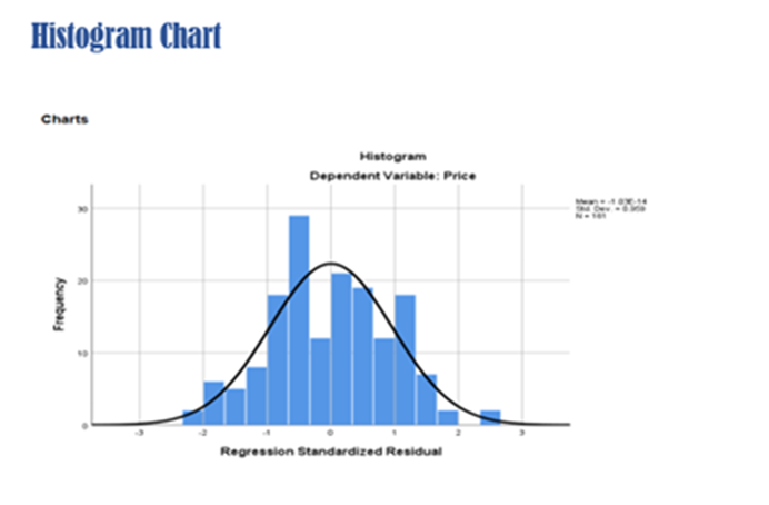
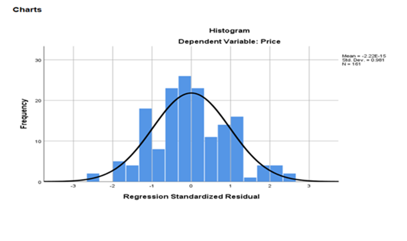
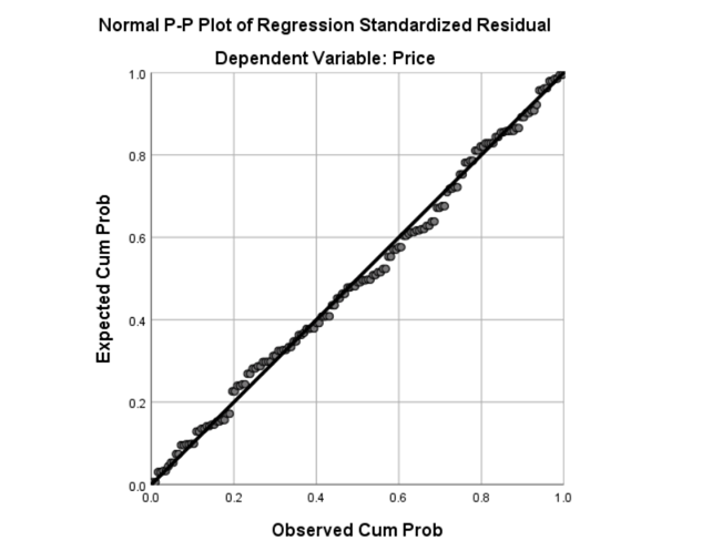
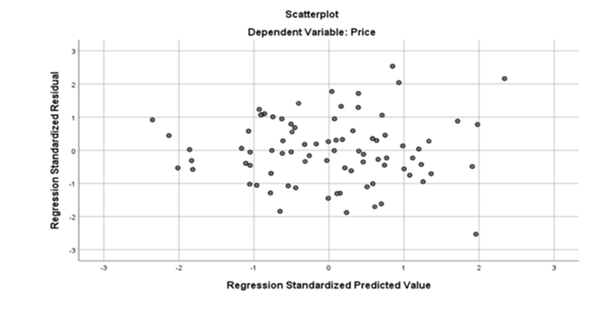
HISTOGRAM
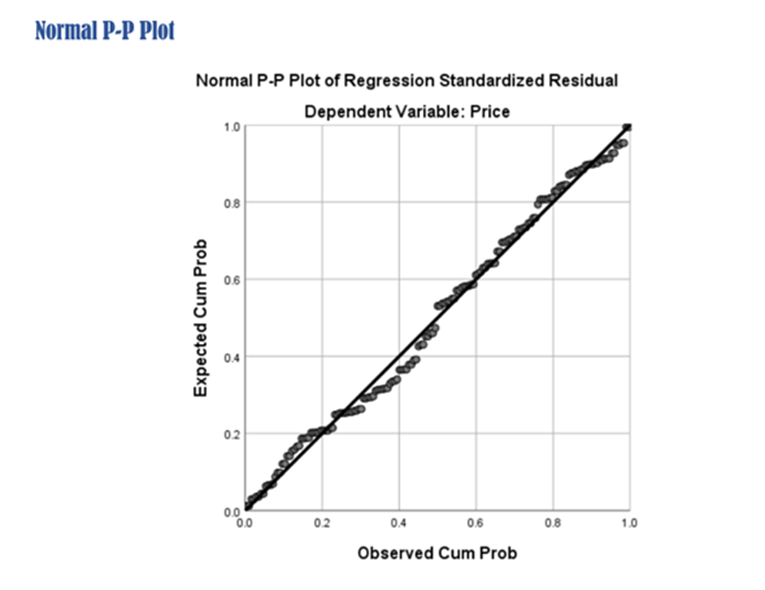
Normal P-P Plot
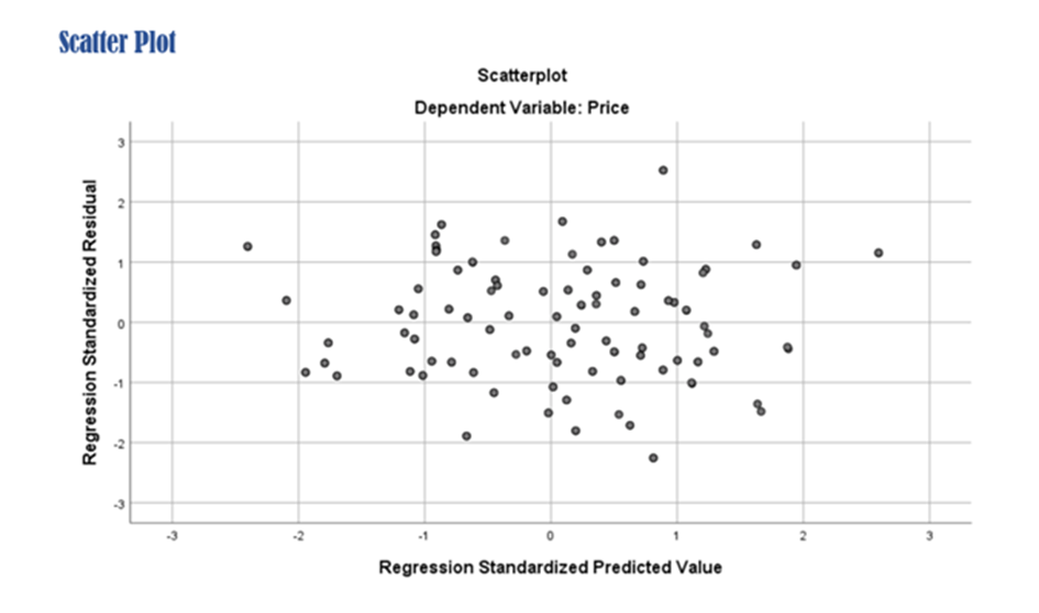
Scatter plot
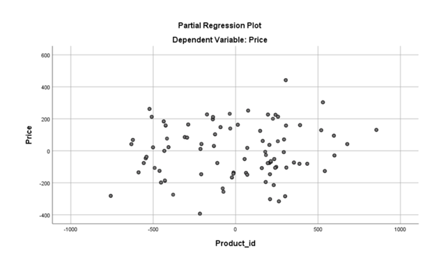
Partial Regression Plot
Methods Used in SPSS
- ENTER
- STEP-WISE
- REMOVE
- BACKWARD
- FORWARD
PARTIAL F-TEST and Variable Selection
- Partial F-Test is important test.
- It is done in Step-Wise Regression Model Building
- The need for this test is required when we check if the additional independent variables add value in the explanation of response variable
- First, we test a model with large number of independent variables
- Second, we test another model with lesser number of independent variables
- We use Partial F-test in selecting new variables with a strategy Step-Wise Regression
- Initially we have K explanatory variables
- In the reduced model we have r explanatory variables where r is less than k. Our Null hypothesis r+1, r+2, r+3, r+4 … k = 0
- All explanatory variables which are not present in the reduced model the beta values are assumed to be zero
Nested Models
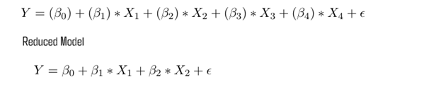
Full model
Reduced Model
The first equation is related to full model containing 13 predictor variables and one intercept The second equation is related to the reduced model containing only 6 predictor variables and one intercept. We have to understand if additional variables add value to the equation and explain the changes in y-dependent variable. To determine if these two models are significantly different, we can perform a partial F-test. A partial F-test calculates the following F test-statistic
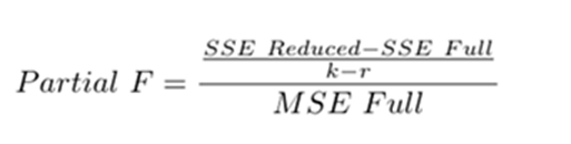
Where:
- SSE [full] Sum of squares of Error(residuals) full model
- SSE[Reduced] Sum of squares of Error(residuals) Reduced model
- k Total number observations in the full dataset
- r number of variables in the reduced model
Sum of squares of residuals will always be smaller for the full model
Since adding predictor variables will always lead to some reduction in error
A partial F-test tests whether the group of predictors that you removed from full model are actually useful and need to be included in the full model
Partial F-test uses the following null and alternate hypothesis
- H0 All coefficients removed from the full model are zero
- HA At least one of the coefficients removed from the full model is non-zero
If the p-value corresponding to the F test-statistic is below a certain significance level (e.g. 0.05), then we can reject the null hypothesis and conclude that at least one of the coefficients removed from the full model is significant. Example
Full model: price = 1720.152+0.031*product_id -0.023*sale -0.563*weight-70.758*resolution
+1.004*ppi +53.517*cpu core +129.577*cpu freq +6.107*internal mem
+91.549*ram + 4.458*RearCam+9.313*Front_cam+1.34*battery-73.605*thickness
n = 161
k =13
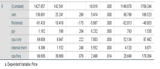
Reduced model: price = 1427.657+136.661*ram-61.433*thickness +1.162*ppi+
69.808*cpu core+6.396*internal mem+99.7606*cpu freq
r=6
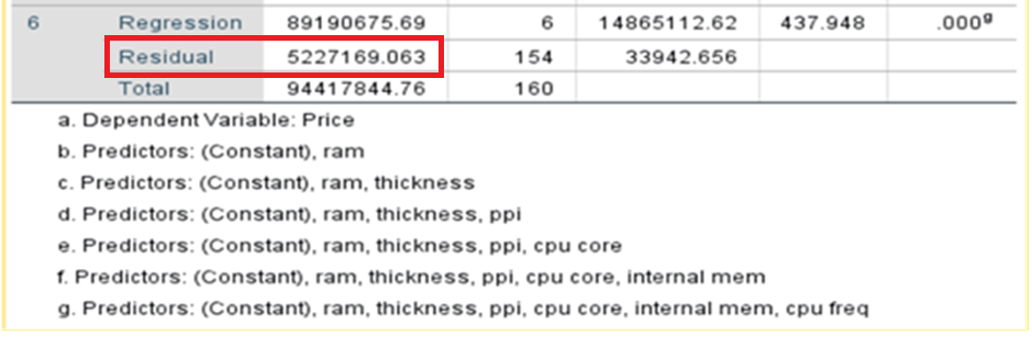
SSE full = 4315775.476
SSR reduced = 5227169.063
MSE Full =29359.017
Partial F-test = (SSE reduced– SSE full/(13-6))/MSE Full
= (5227169.063-4315775.476)/ 7/ 29359.017
=4.43472
P-value for F test statistic
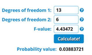
If the p-value corresponding to the F test-statistic is below a certain significance level (e.g. 0.05), then we can reject the null hypothesis and conclude that at least one of the coefficients removed from the full model is significant. We can do some refinement by adding some removed variables and test if they add any value in the explanation of changes in y.
Under Backward Method
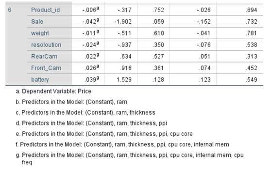
Initially all given 13 independent variables are included and by backward elimination process three variables have been removed based on criteria.
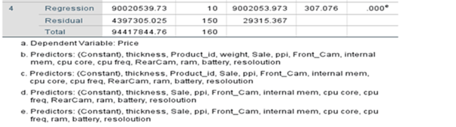
Ten variables have been selected
SSE full = 4315775.476
SSR reduced = 4397305.025
MSE Full =29359.017
Partial F-test = (SSE reduced– SSE full/(13-10))/MSE Full
= (4397305.025-4315775.476)/ 3/ 29359.017
= 0.92566166
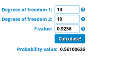
If the p-value corresponding to the F test-statistic is greater than (e.g. 0.05), then we have to accept the null hypothesis and conclude that the added variables do not add any value in the explanation of changes in y and the removal of like product_id, RearCam, and weight is justified.
2.Step-Wise Method
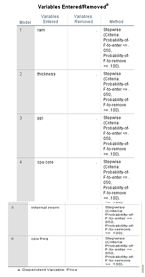
model summary
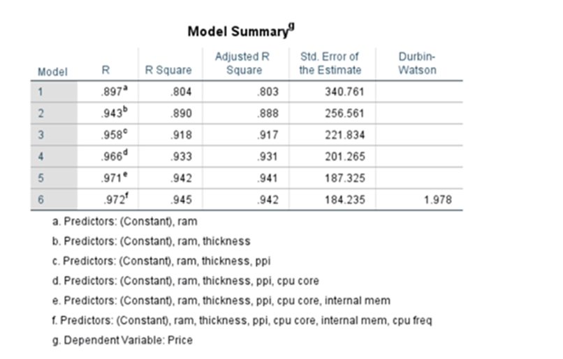
Under step-wise method system provides the coefficients after adding and removing variables based on the conditions set ( cut off 0.05. if p-value of the particular feature falls below that particular variable will be added to the equation and cut off 0.10 if p-value of the particular feature moves above 0.10 the particular variable will be dropped.). System has run 6 steps and finally gives the coefficients which are all less than 0.05.
Yhat = 1427.657+136.661*ram-61.433*thickness +1.162*ppi+69.808*cpu core+6.396*internal mem+99.606*cpu freq
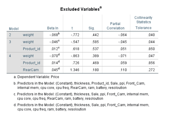
Excluded Variables
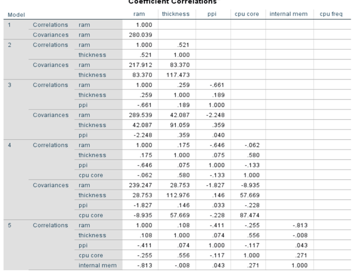
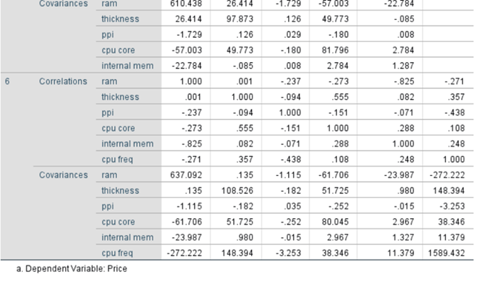
Coefficient Correlations:
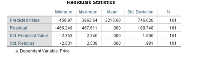
Residual Statistics
Charts:
3.Backward Method:
4:Forward Method
Coefficients
Excluded variables
Dummy Variables for Qualitative Variables in Regression Model
Can we incorporate Qualitative variables in Regression model Building? Yes. Regression model can have qualitative variables like marital status, Say married status categories could be 1) Married 2) Unmarried and 3) divorced. In this case if we add three columns with different betas. it may not look nice for analysis purpose. Whenever, I find qualitative variables I have to convert them using dummy variables or indicator variables. Dummy variables are binary variables. Usually takes 0 or 1.
Can I create n dummy variables? No. When we have n categorical codes we have to create n-1 dummy variables and Beta 0. To avoid dummy variable trap we can have n-1 dummy variables and intercept/beta 0. The intercept/Beta 0 is the base category. When creating dummy variables, we have to leave one category as base category. The remaining coefficients attached to the dummy variables are called differential intercept coefficient, and they measure deviation from the base category for that specific dummy variable.
Interaction Variable
Plays important role in regression model building. You can derive a new variable from the existing variables. In two ways you can derive variables.
First Approach: By taking ratios(say X1(currentAsset) and X2 (Current Liabilities) are variables then you can derive a new variable X3 (Current Ratio) as X1 /X2. Division
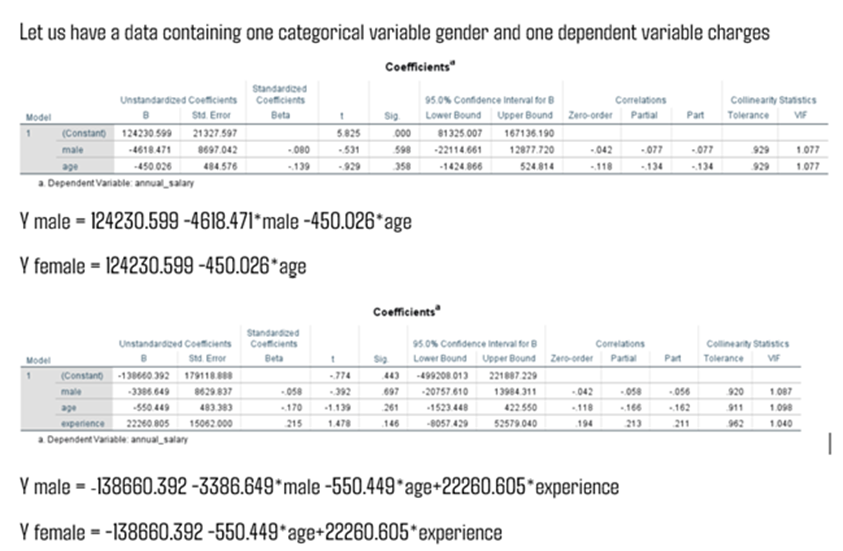
Second Approach: Adopting Interaction Variable. Say Y = β0 + β1X1 + β2X2 + β3X1X2. X1 is Gender and X2 is Work Experience and X1X2 which is wage. product of X1 and X2. Product of quantitative variable and qualitative variable. Multiplication of variables
You can also set Female as 1 and Male as 0. In that case