Convert data into dataframe using pd.DataFrame(already read data). Since we have only one dependent variable (y) and one independent variable (X).Drop the dependent variable from the dataframe and assign it to X.Create the column of Dependent variable and assign it to y.Now change the type of X and y using numpy (np.float64)


Add Constant & iterate:
Results without a constant. Add constant and find results using second iteration

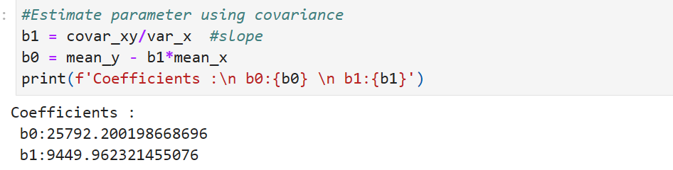
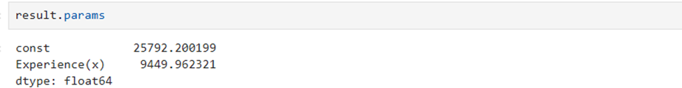
Estimated parameters(Coefficients):

Equations:
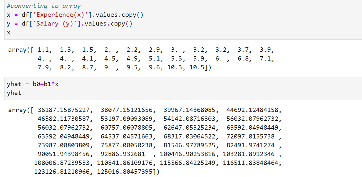
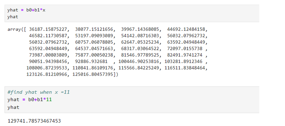
Y hat = 25792.20+9449.96*X
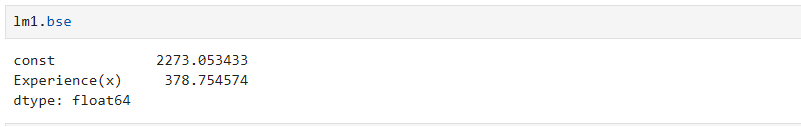

Standard Error of constant and other independent variables:

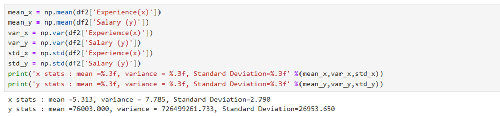
Mean, Variance, and Standard Deviation of X and Y

Covariance(X,y)

Estimation of coefficients(Parameters) Using covariance
Find R-Square using SST,SSR,SSE
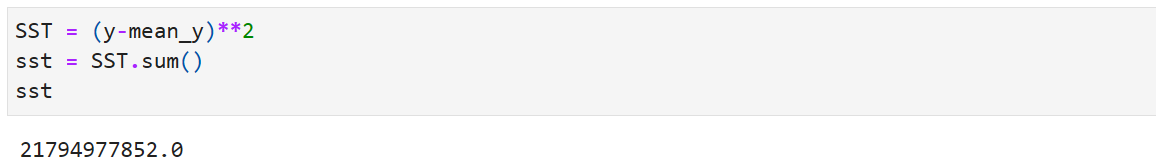
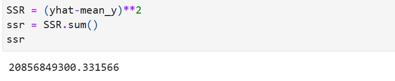
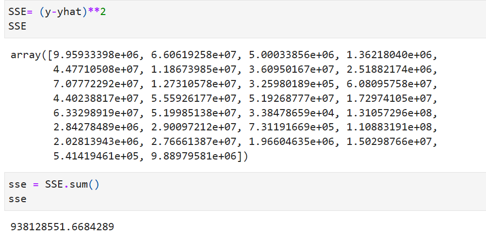
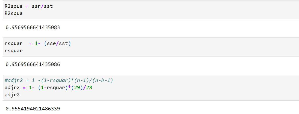
R^2 Calculation:
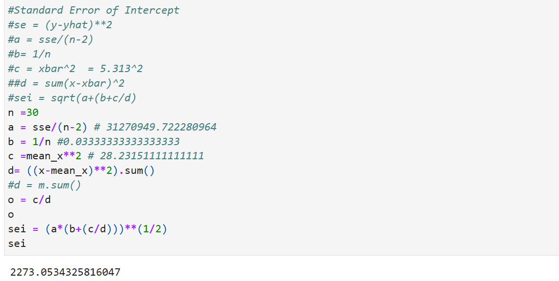
Standard Error of Intercept:
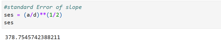
Standard Error of Slope
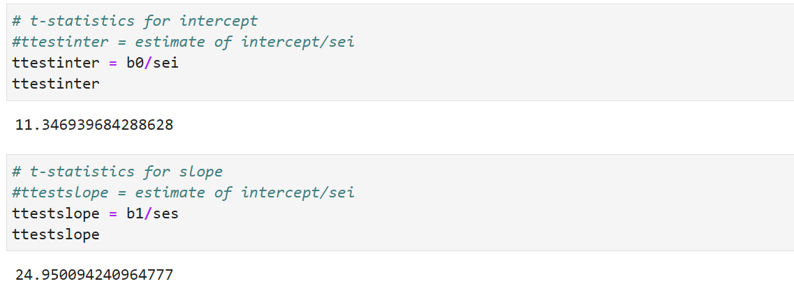
t-statistics for intercept and slope
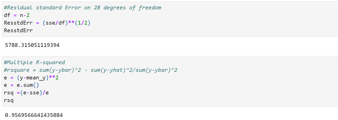
Residual Standard Error
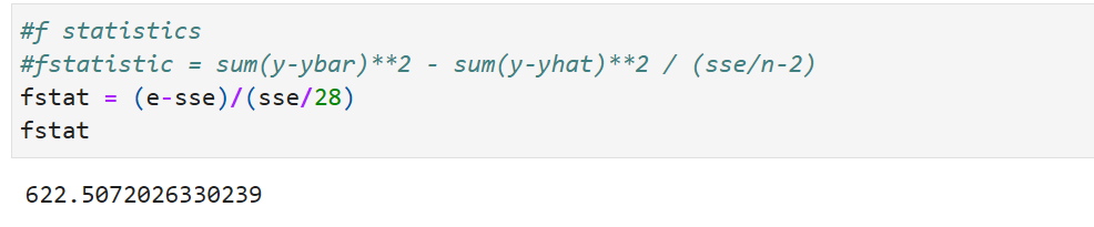
F-statistics
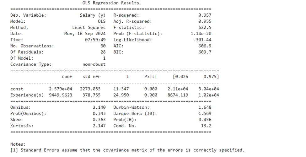
Interpretation of second summary report(lm1.summary())
Part 1
 ummary Part I
provides :
- Dependent Variable : here Salary (y)
- Model Used : We use OLS ( Ordinary Least Square Method)
- Method used : Least Square
- Date and time : The Date and time on which the report was generated
- No.of Observations: Count of the data handled (n)
- Degrees of Freedom Residuals = n-2 = 30-2 =28 = n-k-1 (k is no of predicting variables)
- Degrees of Freedom Model = 1 (one predicting variable)
- Covariance type : nonrobust: Covariance is a measure denotes how the two variables are linked in a positive or negative manner. Robust covariance is calculated in such a way to minimize or elimate the variables. Nonrobust Covariance does not do that as we have only one independent variable in this example.
- The Linear Equation Y hat = 25792.20+9449.96*X explains changes of y (dependent value) when one unit of independent variable changes.
- when one unit of changes in X trys to change 9449.96 times of y. The slope parameter value (9449.96) points out than when one unit of X increases the y will increase by 9449.96 times.
- R-Square is an important measure. works out to 0.957. When express in percentage it works to 95.7%. Our model explains 95.7% of changes in independent variable is explained. The higher the percentage the better the line fit (that is equation found out). R² is a goodness-of-fit measure for linear regression models.Formula R^2 = Sum of Squares of Residuals/Sum of Squares of Total = SSR/SST. Can also be calculated using Sum of Squares of Error. R^2 = 1- SSE/SST
- Adjusted R-square; Whenever, we add an explanatory/independent variable R-Square is used to increase. The resule of our prediction will remain unstable. In order to increase the efficacy of our model Adjusted R-Square was found, which is an extension of R-Square. It will always be less than or equal to R-Square. Formula used Adj R^2 = 1 – ((1-R^2)*(n-1)/(n-k-1)),It penalizes the model for adding irrelevant variables. Useful for comparing models with different number of predictors(Independent variables)
- F-Statistic: It is useful for testing if the overall regression model is a good fit for data undertaken. A higher F-Statistic value means that the model is statistically significant. F-Statistic = Mean Squared Regression /Mean Squared Error. Represents the probability that the observed data would occur by chance.
- F-pvalue : Lower p-value (typically < 0.05) indicates strong evidence against the null hypothesis, meaning the model is significant. Here we reject Null hypothesis. If p-value is greater than 0.05 then accept the Null Hypothesis
- Log Likelihood(Log llf):Measures the likelihood of observing the data given the model. The higher the value, the better the model fits the data. No direct formula. Calculated from the likelihood function, which evaluates the probability of observing the data given the parameter estimates. However, in python (model.llf)
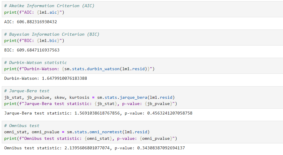
- Akaike Information Criterion(AIC): Quality measure of the model based on the likelihood function. But penalizes models for having too many parameters in multiple linear regression problems Lower AIC is appreciable.
- Bayesian Information Criterion(BIC): Similar to AIC it also penalizes the models having too many parameters. Lower BIC is appreciable.
Part II

Coef: This column displays the value of coefficients(parameters) for the model. yhat = b0 + b1*X. Y hat = 25792.20+9449.96*X Parameters can be found using standard normal equations. In python print(model.params) or model.coef_ and model.intercept_ commands
Std Err: Std Err of Intercept and Std Err of slope can be found as shown above. sei and ses
t : t-Test values for intercept and slope. These are computed as shown above. ttestinter = b0/sei and ttestslope = b1/ses
ttestp-value : this is found using scipy.stats. from scipy.stats import t and then find pvalinter = t.sf(np.abs(b0/sei),28)*2 and pvalslope = t.sf(np.abs(b1/ses)*2. Both are less than <0.05. There is strong evidence against null hypothesis. So we reject null hypothesis and come to conclusion that Experience(x) is statistically significant. Since the p value is less than 0.05 the coefficient relating to Experience(X) is correctly arrived (using t test)
0.025 0.975: the lower and upper bounds of a 95% confidence interval
Part III
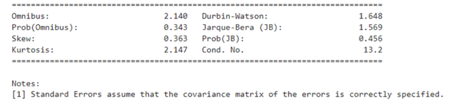
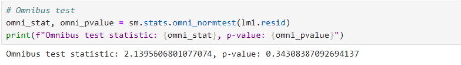
Omnibus: Tests the skewness and kurtosis of the residuals jointly to assess normality. A high statistic indicates that the residuals are not normally distributed. here it comes to 2.140. Prob(omnibus) : 0.343
Durbin_Watson: Tests for autocorrelation in the residuals. Values close to 2 indicate no autocorrelation; values closer to 0 or 4 indicate positive or negative autocorrelation, respectively. here it comes to 1.648 which is less than 2. So there is no autocorrelation. Calculated using

Jarque-Bera Test: Tests whether the residuals follow a normal . A significant Jarque-Bera statistic indicates non-normality. Since p value is not significane (greater than 0.05) we can come to conclustion that the resisduals follow a normal distribution

Condition No: Return condition number of exogenous matrix. Calculated as ratio of largest to smallest singular value of the exogenous variables(X) This value is the same as the square root of the ratio of the largest to smallest eigenvalue of the inner-product of the exogenous variables.
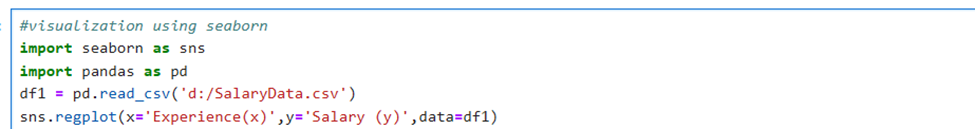
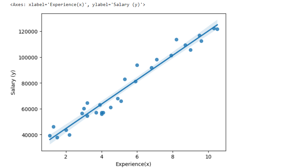
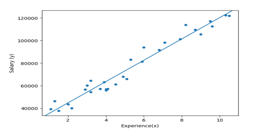
Visualization using seaborn library
Using statsmodels.abline_plot():
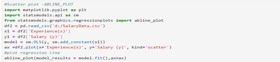
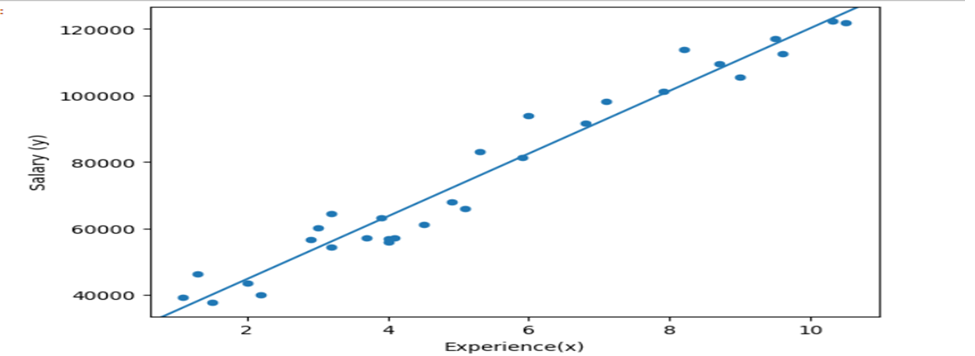


Parameters:


px.scatter:


DESCRIPTIVE STATISTICS:
COVARIANCE:

REGRESSION COEFFICIENTS:

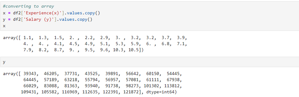
CONVERSION TO ARRAY:
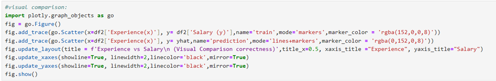
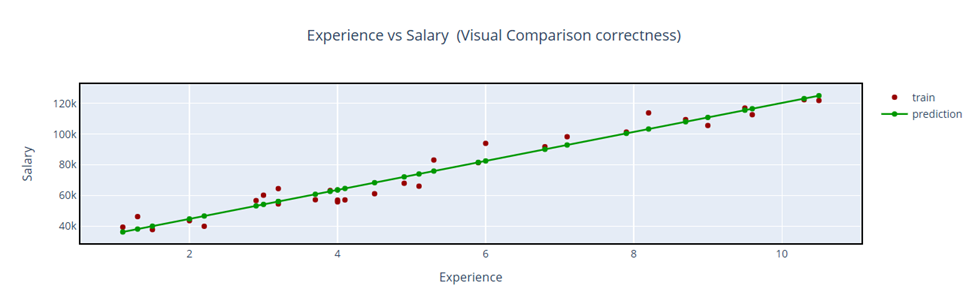
Visual comparison- using Plotly.graph_objects