- Raw Data is collected using Observations/when conducting experiment
- Individual observations could be called Random Variable X
- How many times the same value occurs is called frequency
- Using a tally-sheet you can calculate the frequency of observations from the raw data
- Primary data are not arranged in a tabular form
- A tally-mark (/ or |) is put against the value when it occurs in the raw data
Let us see the data that shows 50 students marks
|
Marks x |
Marks x | Marks x | Marks x |
Marks x |
|
37 |
47 | 32 | 26 |
21 |
|
41 |
38 | 41 | 50 |
45 |
|
52 |
46 | 37 | 45 |
31 |
|
40 |
44 | 48 | 46 |
16 |
|
30 |
40 | 36 | 32 |
47 |
|
37 |
47 | 50 | 40 |
45 |
|
51 |
52 | 38 | 26 |
41 |
|
33 |
38 | 39 | 37 |
32 |
|
40 |
38 | 50 | 38 |
48 |
|
41 |
36 | 41 | 41 |
52 |
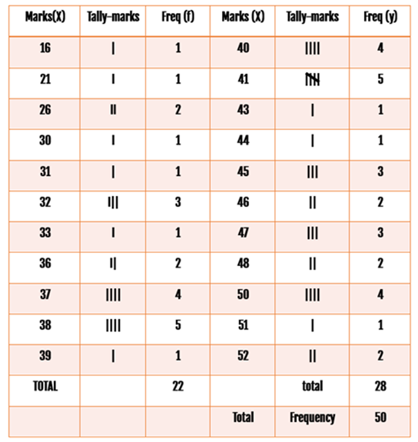
Such a representation of the data is known as the Frequency Distribution
Rules for making classes:
- The number of classes should neither be too large nor too small.
- It should not exceed 20 but should not be less than 5, normally, depending on the number of observations in the raw data
Group Frequency Distribution:
- Say large masses of raw data are to be summarized using frequency
- The identity of the individual observation or the order in which observations arise are not relevant for the analysis
- We distribute the data into classes or categories and determine the number of individuals belonging to each class, called the class-frequency.
- A tabular arrangement of raw data by classes where the corresponding class-frequencies are indicated is known as Grouped Frequency distribution
Terms associated with Group Frequency Distribution
- Class-interval
- Class-frequency, total frequency
- Class-limits (upper and lower)
- Class boundaries (upper and lower)
- Mid-value of class interval (or class mark)
- Width of class interval
- Frequency density
- Percentage Frequency
Class Limits: The two ends of a class-interval are called class-limits
Class boundaries: obtained from the class limits as follows
- Lower class-boundary = lower class limit – ½ d
- Upper class-boundary = upper class limit + ½ d
- Where d = common difference between upper class of any class-interval with the lower class of the next class-interval. In the table d = 1.
- Lower class boundary =16-1/2*1=16-0.5 = 15.5
- Upper class boundary =20 +1/2*1=20+0.5 = 20.5
- Again, for the next class-interval,
- lower class-boundary = 20.5,
- upper class boundary = 25.5 and so on
Mid Value(Class-mark):
- Mid value : (or class mark).
- It is calculated by adding the two class limits divided by 2.
- In the above table : for the first class-interval
- Mid value = (16+20)/2 = 18
- For next mid value = (21+25)/2 = 23 and so on
Width of Class-Interval:
- Width : The width (or size) of a class interval is the difference between the class-boundaries (not class limits)
- Width = Upper class boundary – lower class boundary
- For the first class, width = 20.5 – 15.5 = 5
- For the second class width = 25.5 – 20.5 = 5, so on
Frequency Density:
Frequency density : It is the ratio of the class frequency to the width of that class-interval i.e.
frequency density = class frequency /width of the class
- For the first- class frequency density = = 1/5 = 0.2
- For the third- class frequency density= = 3/5=0.6
Percentage Frequency:
It is the ratio of class-frequency to total frequency expressed as percentage.
percentage frequency = ´(class frequency *100)/total frequency
In the table for the frequency 5,
% frequency = 5 *100/ 50 = 10
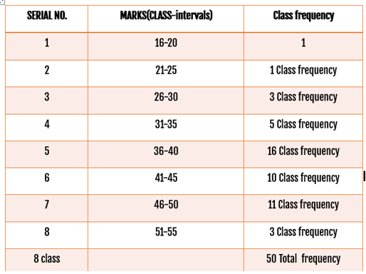
After finding out the frequency of the raw data (50 students marks) using Tally mark let us rearrange the table as shown below based on Class-interval.
Range of the given data: 16-52
Lower class limit = 16,21,26,31,36,41,46,50
Upper class limit = 20,25,30,35,40,45,50,55
Sum of class frequency must be equal to the total number of observations
Class-interval could be either 1) Inclusive Class interval or 2) Exclusive Class Interval
INCLUSIVE CLASS INTERVAL:
Here both Lower-class limit and upper- class limit are included. Say 16 -20. if you have data 15.5 or 20.5 you can’t place tally mark either in 16-20 or 21-25. This is the problem. Because there is a gap between upper-class limit and the next lower-class limit. Many data are omitted. To solve this problem, we have to convert Inclusive class intervals to Exclusive class intervals
The above-said inclusive class interval is converted into Exclusive class interval as shown below
Exclusive Class Interval
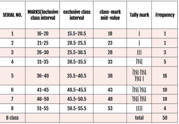
- Upper-class Limit – next lower-class limit = 21-20= 1 (gap)/2 = 0.5
- Lower part is called Lower Class Boundary(LCB)
- upper part is called Upper Class Boundary(UCB)
- Now you can mark 15.5 or 20.5 if data are available.
- Now another problem say 20.5 appears in both 15.5-20.5 and 20.5 -25.5 classes. Where to mark ?
Rule:
- Lower class boundary is included
- upper-class boundary is excluded.
Now 15.5 data is marked in the class interval 15.5-20.5
If you have data 20.5 tally mark is marked in the class interval 20.5-25.5
Important points in creation of Frequency Distribution:
- A frequency distribution : arranges observations in an increasing order
- A frequency distribution of a continuous variable is known as Grouped frequency distribution
- The distribution of shares is an example of frequency distribution of a continuous variable
- Mutually exclusive classification excludes upper class limit but includes lower class limit.
- Mutually inclusive classification is meant for a continuous variable
- Mutually exclusive classification is meant for an attribute
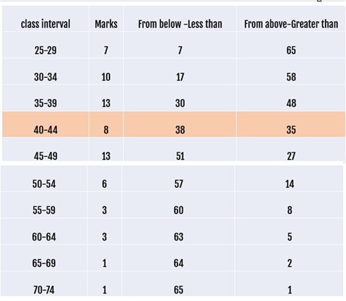
Cumulative Frequency Distribution:
- Here the frequencies are cumulated.
- This is prepared from a grouped frequency distribution showing the class boundaries by adding each frequency to the total of the previous one.
- By adding each frequency those following it.
- The former is termed as Cumulative frequency of less than type
- The latter, the cumulative frequency of greater than type
Let us have the following mathematics marks of 65 students in a school
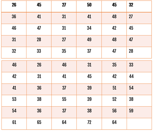
Minimum : 26 Maximum : 72 range = 72-26 = 46
Let us find frequency using tally marks using inclusive class interval
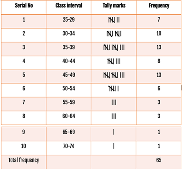
- The LCB is a lower limit to LCL. LCL –D/2
- D is length of UCL-NEXT LCL = 30-29 = 1
- LCB = 25-(30-29)/2 = 24.5
- The UCB is upper limit to UCL
- UCB = 29+(30-29)/2 =29.5
- The length/size of a class is
- difference between UCB and LCB
- For particular class boundary, the less than cumulative frequency and more than cumulative frequency add up to – none
- frequency density corresponding to a class interval is the ratio of class frequency to the total frequency
- Relative frequency for a particular class lies between 0 and 1
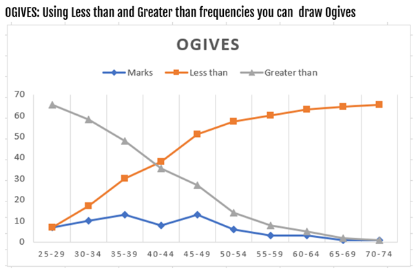
OGIVE of cumulative frequency polygon:
If the cumulative frequencies are plotted against the class boundaries and successive points are joined by straight lines, we get what is known as Ogive (or cumulative frequency polygon).
There are two types of Ogive.
- Less than type – Cumulative Frequency from below are plotted against the upper class-boundaries. This is known as less than type, because the ordinate of any point on the curve (obtained) indicates the frequency of all values less than
- Greater than type – Cumulative frequencies from above are plotted corresponding lower boundaries. or equal to the corresponding value of the variable represented by the abscissa of the point. This is known as the greater than type
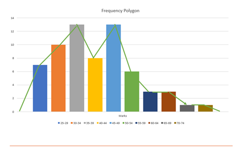
Frequency Polygon via Histogram:
- Draw histogram first
- then joining all the midpoints of the tops (upper side) of the adjacent rectangle of the histogram by straight line graphs.
The figure so obtained is called a frequency polygon. It is necessary to close the polygon at both ends by extending them to the base line so that it meets the X-axis at the mid points of the two hypothetical classes i.e. the class before the first class & the class after the last class having the zero frequency.